Standard Pivot Tables have a simple feature for creating calculated items. You can think of a calculated item as “virtual rows” in the source data. A calculated item will not appear in the field list window. Instead, it will appear as an item in the field for which it is defined. In the example shown, a calculated item called “Southeast” has been created with a formula that adds South to East. The pivot table displays the correct regional totals, including the new region “Southeast”.
Fields
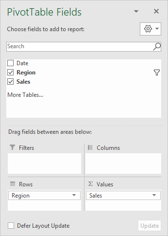
The source data contains three fields: Date, Region, and Sales. Note the field list does not include the calculated item.
The calculated item was created by selecting “Insert Calculated Item” in the “Fields, Items, and Sets” menu on the ribbon:
<img loading=“lazy” src=“https://exceljet.net/sites/default/files/images/pivot/inline/pivot%20table%20calculated%20item%20ribbon%20menu.png" onerror=“this.onerror=null;this.src=‘https://blogger.googleusercontent.com/img/a/AVvXsEhe7F7TRXHtjiKvHb5vS7DmnxvpHiDyoYyYvm1nHB3Qp2_w3BnM6A2eq4v7FYxCC9bfZt3a9vIMtAYEKUiaDQbHMg-ViyGmRIj39MLp0bGFfgfYw1Dc9q_H-T0wiTm3l0Uq42dETrN9eC8aGJ9_IORZsxST1AcLR7np1koOfcc7tnHa4S8Mwz_xD9d0=s16000';" alt=“Select “Insert calculated Item” from this menu - 2”>
The calculated field is named “Southeast” and defined with the formula “=South + East” as seen below:
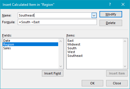
Note: Field names with spaces must be wrapped in single quotes (’). Excel will add these automatically when you click the Insert Field button or double-click a field in the list.
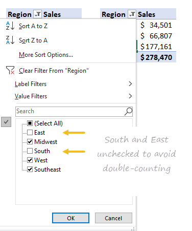
After the calculated item is created, the East and South regions must be excluded with a filter to avoid double-counting:
Steps
- Create a pivot table
- Add Region as a Row field
- Add Sales as a Value field
- Create the Calculated item “Southeast”
- Filter Region to exclude East and South
To apply conditional formatting to a pivot table, create a new conditional formatting rule and pay particular attention to the “apply rule to” settings as described below. In the example shown, there are two rules applied. The green shows the top 5 values using a rule like this:

Details
Pivot tables are dynamic and change frequently when data is updated. If you created conditional formatting rules based on “selected cells” only, you may find that the conditional formatting is lost or not applied to all data when the pivot table is changed, or when data is refreshed.
The best option is to set up the rule correctly from the start. Select any cell in the data you wish to format and then choose “New rule” from the conditional formatting menu on the Home tab of the ribbon. At the top of the window, you will see a setting for which cells to apply conditional formatting to. For the example shown, we want the last option: All cells showing “Sum of sales” values for “Name” and “Date”.

Note: The second option, “All cells showing “Sum of Sales values”, will include grand total rows and columns as well, which you ordinarily don’t want.
Editing existing rules to fix broken formatting
If you already have a rule set up that is not correctly formatting all values as needed, edit the rule and change the cell selection option if needed. You can access existing rules at Home > Conditional Formatting > Manage Rules.
In the example shown, the rule manager displays two rules like this:

To edit a rule, select the rule and click the “Edit Rule” button. Then adjust settings in the “Apply rule to” section.
Note: conditional formatting is lost when you remove the target field from a pivot table.
