A pivot table is an easy way to count blank values in a data set. In the example shown, the source data is a list of 50 employees, and some employees are not assigned to a department. The Pivot Table is configured to group out data by department, and automatically creates a category called “(blank)” for employees without a department value.
Fields
The pivot table shown is based on three fields: First, Last, and Department. The Department field is configured as a Row field, and Last is configured as a Value field, renamed “Count”.
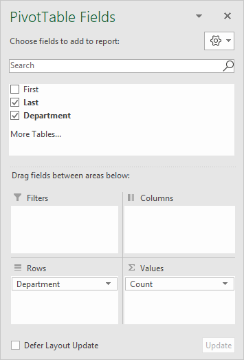
The Last field is renamed “Count” and configured to summarize by count:
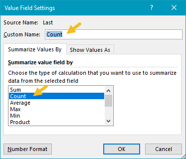
In the example shown, the pivot table uses the Last field to generate a count. Any text field in the data that is guaranteed to have data can be used to calculate count.
Steps
- Create a pivot table
- Add Department field to the rows area
- Add Last field Values area
Notes
- Any non-blank field in the data can be used in the Values area to get a count.
- When a text field is added as a Value field, Excel will display a count automatically.
Pivot tables have a built-in feature to group dates by year, month, and quarter. In the example shown, a pivot table is used to count colors per month for data that covers a 6-month period. The count displayed represents the number of records per month for each color.
Fields
The source data contains three fields: Date , Sales , and Color . Only two fields are used to create the pivot table: Date and Color .

The Color field has been added as a Row field to group data by color. The Color field has also been added as a Value field, and renamed “Count”:

The Date field has been added as a Column field and grouped by month:

Helper column alternative
As an alternative to automatic date grouping, you can add a helper column to the source data, and use a formula to extract the year . Then add the Year field to the pivot table directly.
COUNTIFS alternative
As an alternative to a pivot table, you can use the COUNTIFS function to count by month, as seen in this example .
Steps
- Create a pivot table
- Add Color field to Rows area
- Add Color field Values area, rename to “Count”
- Add Date field to Columns area, group by Month
- Change value field settings to show count if needed
Notes
- Any non-blank field in the data can be used in the Values area to get a count.
- When a text field is added as a Value field, Excel will display a count automatically.
- Without a Row field, the count represents all data records.
