Pivot Table Count With Percentage

To display data in categories with a count and percentage breakdown, you can use a pivot table. In the example shown, the field “Last” has been added as a value field twice – once to show count, once to show percentage. The pivot table shows the count of employees in each department along with a percentage breakdown.

Fields

The pivot table shown is based on two fields: Department and Last . The Department field is configured as a Row field, and the Last field is a Value field, added twice:

The Last field has been added twice as a value field. The first instance has been renamed “Count”, and set summarize by count:

The second instance has been renamed to “%”. The summarize value setting is also Count, Show Values As is set to percentage of grand total:

Steps

1. Create a pivot table
2. Add Department as a Row field
3. Add Last as a Value field Rename to “Count” Summarize by Count
4. Add Last as a Value field Rename to “%” Summarize by Count Display Percent of Grand Total Change number formatting to percentage

When a filter is applied to a Pivot Table, you may see rows or columns disappear. This is because pivot tables, by default, display only items that contain data. In the example shown, a filter has been applied to exclude the East region. Normally the Blue column would disappear, because there are no entries for Blue in the North or West regions. However, Blue remains visible because field settings for color have been set to “show items with no data”, as explained below.

Fields

The pivot table shown is based on three fields: Region, Color, and Sales:

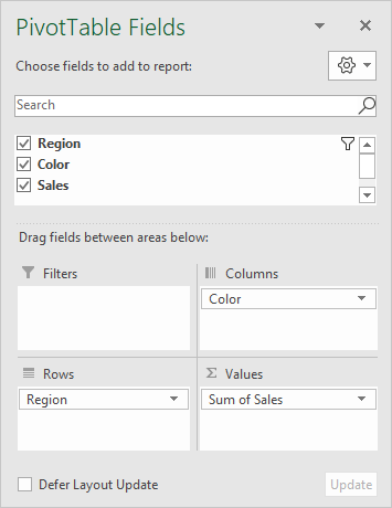
Region has been configured as a Row field, Color as a Column field, and Sales is a Value field.

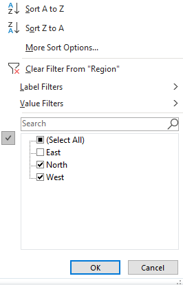
Data has been filtered by Region to exclude East:

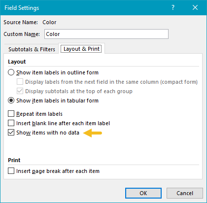
To force the display of items with no data, “Show items with no data” has been enabled on the Layout & Print tab of the Color field settings, as seen below:

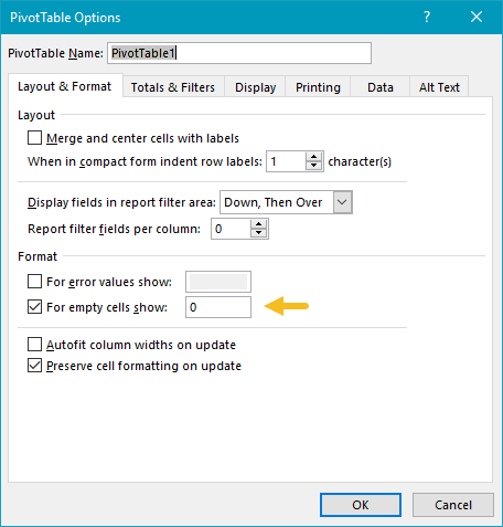
To force the pivot table to display zero when items have no data, a zero is entered in general pivot table options:

Finally, the Accounting number format has been applied to the Sales field to display empty cells with a dash (-).

Note: the same problem can occur with dates are grouped as months, and no data appears in a given month. You can use the same approach, with a few extra steps, described here .

Steps

1. Create a pivot table
2. Add Region field to Rows area
3. Add Color field to Columns area Enable “show items with no data”
4. Add Sales field to Values area Apply Accounting number format
5. Set pivot table options to use zero for empty cells