Pivot Table Filter By Weekday

To create a pivot table with a filter for day of week (i.e. filter on Mondays, Tuesdays, Wednesdays, etc.) you can add a helper column to the source data with a formula to add the weekday name, then use the helper column to filter the data in the pivot table. In the example shown, the pivot table is configured to show data for Mondays only.

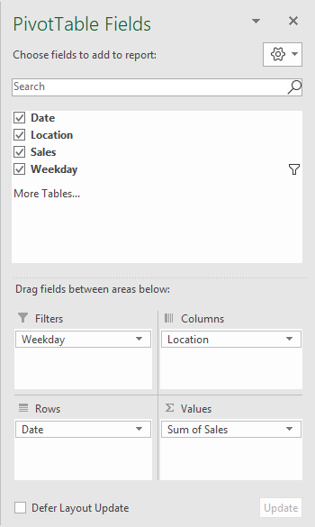
Pivot Table Fields

In the pivot table shown, there are four fields in use: Date, Location, Sales, and Weekday. Date is a Row field, Location is a Column field, Sales is a Value field, and Weekday (the helper column) is a Filter field, as seen below. The filter is set to include Mondays only.

Helper Formula

The formula used in E5, copied down, is:

=TEXT(B5,"ddd")

This formula uses the TEXT function and a custom number format to display an abbreviated day of week.

Steps

1. Add helper column with formula to data as shown
2. Create a pivot table
3. Add fields to Row, Column, and Value areas
4. Add helper column as a Filter
5. Set filter to include weekday(s) as needed

Notes

1. You can use the helper column to group by weekday as well

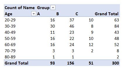
Pivot tables have a built-in feature to group numbers into buckets at a given interval. In the example shown, a pivot table is used to group a list of 300 names into age brackets separated by 10 years. This numeric grouping is fully automatic.

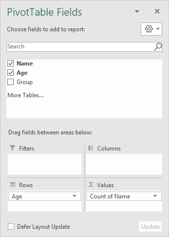
Fields

The source data contains three fields: Name, Age, and Group. Only Name and Age are used in the pivot table as shown:

Age is used as a Row field. After Age has been added to the pivot table, it has been grouped as below:

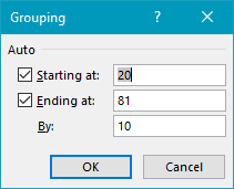
Starting and ending value are automatically entered based on the source data. The “by” is set to 10 years, but can be customized as needed.

The pivot table maintains age grouping when fields are added or reconfigured. For example, when the Group field is added as a Column field, the pivot table below is created:

Steps

1. Create a pivot table
2. Add Age as a Row field
3. Add Name as a Value field
4. Group Age into buckets of 10 years