To group a pivot table by day of week (e.g. Mon, Tue, Wed, etc.) you can add a helper column to the source data with a formula to extract the weekday name, then use the helper to group data in the pivot table. In the example shown, the pivot table is configured to display sales by weekday. Note that Excel automatically sorts standard weekday names in a natural order, instead of alphabetically.
Pivot Table Fields
In the pivot table shown, there are four fields in use: Date, Area, Sales, and Day. Three of these fields are used to create the pivot table shown: Area is a Row field, Day is a Column field, and Sales is a Value field, as seen below.
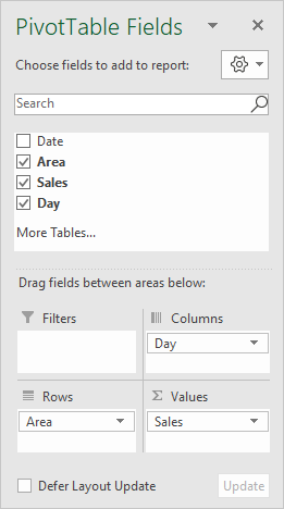
When the Sales field is first added as a Value field, it is automatically named “Sum of Sales”. In the example, it has been renamed “Sales “, with a trailing space to prevent Excel from complaining that the name is already in use.
<img loading=“lazy” src=“https://exceljet.net/sites/default/files/images/pivot/inline/pivot%20table%20group%20by%20day%20of%20week%20value%20field%20settings.png" onerror=“this.onerror=null;this.src=‘https://blogger.googleusercontent.com/img/a/AVvXsEhe7F7TRXHtjiKvHb5vS7DmnxvpHiDyoYyYvm1nHB3Qp2_w3BnM6A2eq4v7FYxCC9bfZt3a9vIMtAYEKUiaDQbHMg-ViyGmRIj39MLp0bGFfgfYw1Dc9q_H-T0wiTm3l0Uq42dETrN9eC8aGJ9_IORZsxST1AcLR7np1koOfcc7tnHa4S8Mwz_xD9d0=s16000';" alt=“Sales field renamed to “Sales " - 2”>
Helper Formula
The formula used in E5, copied down, is:
=TEXT(B5,"ddd")
This formula uses the TEXT function and a custom number format to display an abbreviated day of week.
Steps
- Add helper column with the formula above as shown
- Create a pivot table
- Drag Day to the Columns area
- Drag Area to the Rows area
- Drag Sales to the Values area Rename to “Sales " (note trailing space)
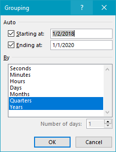
Pivot tables have a built-in feature to group dates by year, month, and quarter. In the example shown, a pivot table is used to summarize sales by year and quarter. Once the date field is grouped into years and quarters, the grouping fields can be dragged into separate areas, as seen in the example.
Fields
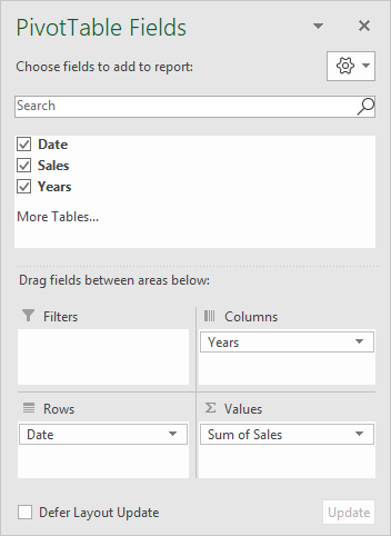
The source data contains two fields: Date, and Sales, and both are used create the pivot table, along with Years, which appears after dates are grouped:
The Date field has been grouped by Years and Quarters:
After grouping, the Years field appears in the field list, and the Date field displays quarters in the form “Qtr1”, “Qtr2”, etc. Years has been added as a Column field, and Date (Quarters) has been added as a Row field.
Finally, the Sales field has been added as a Value field, and set to Sum values:
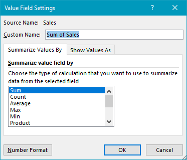
and the number format has been set to display currency.
Helper column alternative
As an alternative to automatic date grouping, you can add helper columns to the source data, and use a formula to extract the year , and another formula to create a value for Quarter . This allows you to assign custom abbreviations to quarters, and to calculate fiscal year quarters that don’t begin in January if needed. Once you have these values in helper columns, you can add them directly to the pivot table without grouping dates.
Steps
- Create a pivot table
- Add Date as a Column field, group by Years and Quarters
- Move Date (Quarters) to Rows area
- Add Sales field to Values area
- Change value field settings to use desired number format
