Pivot tables have a feature to group dates by year, month, and quarter. In the example shown, a pivot table is used to summarize support issues by month and by priority. Each row in the pivot table lists the count of issues recorded in a given month by priority (A, B, C). The Total columns shows the total count of issues recorded in each month.
Note: the source data contains data for an entire year, but the pivot table is filtered to show only the first 6 months of the year, January through June.
Fields
The source data contains three fields: Issue , Date , and Priority . All three fields are used to create the pivot table:
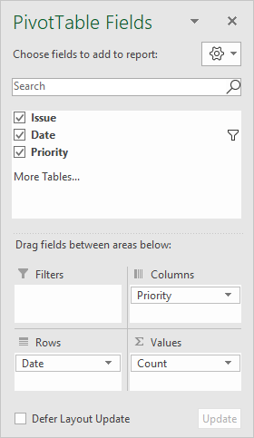
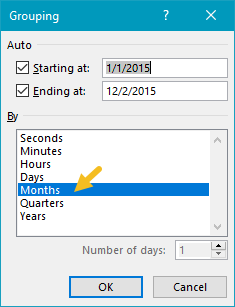
The Date field has been added as a Row field and grouped by month:
The Priority field has been added as a Column field.
The Issue field has been added as a Value field and renamed “Count” for clarity. Because Issue contains text field, the calculation is automatically set to Count:
<img loading=“lazy” src=“https://exceljet.net/sites/default/files/images/pivot/inline/pivot%20table%20issue%20count%20by%20priority%20value%20field%20settings.png" onerror=“this.onerror=null;this.src=‘https://blogger.googleusercontent.com/img/a/AVvXsEhe7F7TRXHtjiKvHb5vS7DmnxvpHiDyoYyYvm1nHB3Qp2_w3BnM6A2eq4v7FYxCC9bfZt3a9vIMtAYEKUiaDQbHMg-ViyGmRIj39MLp0bGFfgfYw1Dc9q_H-T0wiTm3l0Uq42dETrN9eC8aGJ9_IORZsxST1AcLR7np1koOfcc7tnHa4S8Mwz_xD9d0=s16000';" alt=“Value field settings - Issue renamed to “Count” - 3”>
COUNTIFS alternative
As an alternative to a pivot table, you can use the COUNTIFS function to count by month, as seen in this example .
Steps
- Create a pivot table
- Add Date field to Rows area, group by Month
- Add Priority field to Columns area
- Add Issue field Values area, rename to “Count”
Notes
- Any non-blank field in the data can be used in the Values area to get a count.
- When a text field is added as a Value field, Excel will display a count automatically.
- Without a Row field, the count represents all data records.
To create a pivot table that shows the last 12 months of data (i.e. a rolling 12 months), you can add a helper column to the source data with a formula to flag records in the last 12 months, then use the helper column to filter the data in the pivot table. In the example shown, the current date is August 23, 2019, and the pivot table shows 12 months previous. When new data is added over time, the pivot table will continue to track the previous 12 months based on the current date.
Fields
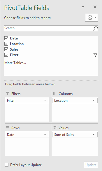
In the pivot table shown, there are three fields in the source data: Date, Sales, and Filter. Filter is a helper column with a formula flagging the last 12 months. The Date field has been grouped by Year and Month:
Formula
The formula used in E5, copied down, is:
=AND(B5>=EOMONTH(TODAY(),-13)+1,B5<EOMONTH(TODAY(),-1))
This formula returns TRUE when a date is greater than or equal to the first day of the month 12 months earlier and when the date is less than the last day of the previous month. The formula uses the AND, TODAY, and EOMONTH functions as explained here .
Steps
- Add helper column with formula to data as shown
- Create a pivot table
- Add Sales as a Value field
- Add Date as a Row field
- Group Date by Year and Month
- Disable subtotals for Year
- Add helper column as a Filter, filter on TRUE
