Pivot Table Latest Values

To build a pivot table that shows latest n values by date, you can add the date as a value field set to show maximum value, then (optionally) add a field as a row column and filter by value to show n values. In the example shown, Date is a value field set to Max, and Sales is a Row field filtered by value to show top 1 items.

Pivot Table Fields

In the pivot table shown, there are three fields, Name, Date, and Sales. Name is a Row field, Sales is a Row field filtered by value, and Date is a Value field set to Max.

The Date field settings are set as shown in below. Note the field has been renamed to “Latest” and set to Max:

The Sales field has a Value filter applied to show the top 1 item by Latest (Date):

Steps

1. Create a pivot table
2. Add Row field(s) as needed
3. Add the Date field as a Value field and set to Max (rename if desired)
4. Apply a Value filter to show Top 10 items and customize as needed

To extract a list of unique values from a data set, you can use a pivot table. In the example shown, the color field has been added as a row field. The resulting pivot table (in column D) is a one-column list of unique color values.

Data

The data in this pivot tables comes from the Excel Table in column B. Excel Tables are dynamic and will automatically expand and contract as values are added or removed. This allows the Pivot Table to always show the latest list of unique values (after refresh).

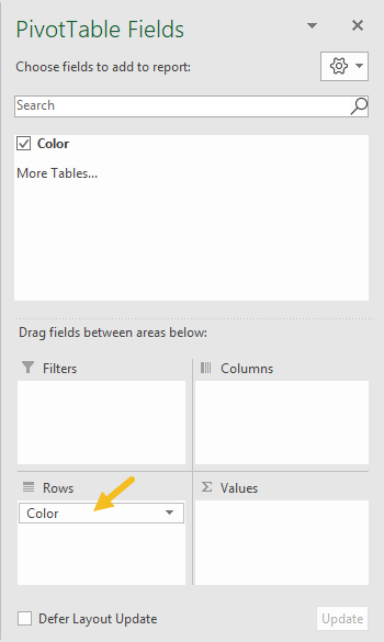
Fields

The pivot table shown in the example has just one field in the row area, as seen below.

Steps

1. Define an Excel Table (optional)
2. Create a Pivot Table (Insert > Pivot Table)
3. Add the color field to the Rows area
4. Disable Grand Totals for rows and columns
5. Change layout to Tabular (optional)
6. When data changes, Refresh pivot Table for latest list.