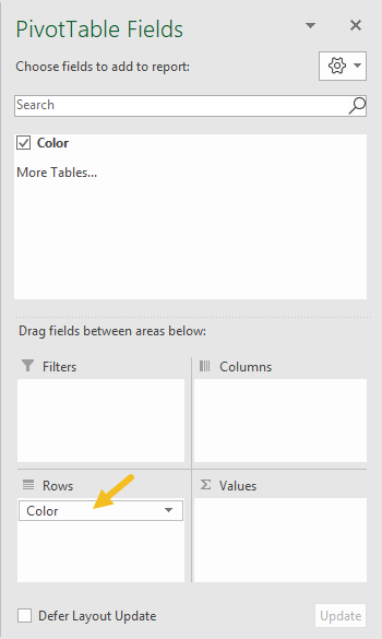
To extract a list of unique values from a data set, you can use a pivot table. In the example shown, the color field has been added as a row field. The resulting pivot table (in column D) is a one-column list of unique color values.
Data
The data in this pivot tables comes from the Excel Table in column B. Excel Tables are dynamic and will automatically expand and contract as values are added or removed. This allows the Pivot Table to always show the latest list of unique values (after refresh).
Fields
The pivot table shown in the example has just one field in the row area, as seen below.
Steps
- Define an Excel Table (optional)
- Create a Pivot Table (Insert > Pivot Table)
- Add the color field to the Rows area
- Disable Grand Totals for rows and columns
- Change layout to Tabular (optional)
- When data changes, Refresh pivot Table for latest list.
In the example shown, a pivot table is used to show the month-over-month variance in sales for each month of a given year. The variance is displayed both as an absolute value and also as a percentage. The year is selected by using a global filter.
Source data
The source data contains three fields: Date, Sales, and Color converted to an Excel Table . Below are the first 10 rows of data:
| Date | Sales | Color |
|---|---|---|
| 1-Jan-2018 | 265 | Silver |
| 2-Jan-2018 | 395 | Green |
| 3-Jan-2018 | 745 | Green |
| 4-Jan-2018 | 665 | Blue |
| 5-Jan-2018 | 565 | Blue |
| 6-Jan-2018 | 145 | Blue |
| 7-Jan-2018 | 115 | Red |
| 8-Jan-2018 | 400 | Green |
| 9-Jan-2018 | 605 | Silver |
| 10-Jan-2018 | 595 | Blue |
Fields
The pivot table uses just two of the three fields in the source data: Date, and Sales. Because Date is grouped by Years and Months, it appears twice in the list, once as “Date” (month grouping), and once as “Years”:

The Date field has been grouped by Months and Years:

The grouping automatically creates a “Years” field, which has been added to the Filters area. The Original “Date” field is configured as a Row field, which breaks down sales by month.
The Sales field has been added to the Values field three times. The first instance is a simple Sum of Sales, renamed to “Sales " (note the extra space at the end):

The second instance of Sales has been renamed “$ Diff”, and set to show a “Difference From” value, based on the previous month:

The third instance of Sales has been renamed “% Diff”, and set to show a “% Difference From” value, based on the previous month:

Steps
- Create a pivot table
- Add the Date field to the Rows area, group by Years and Months
- Set the Rows area to show Date only (month grouping)
- Add Years to the Filter area
- Add Sales to Values area as Sum, rename “Sales "
- Add Sales to Values area, rename to “$ Diff” Show values as = Difference From Base field = Date Base item = Previous
- Add Sales to Values area, rename to “% Diff” Show values as = % Difference From Base field = Date Base item = Previous Set number formatting as desired
- Select the desired year in the Filter
Notes
- When Date is grouped by more than one component (i.e. year and month) field names will appear differently in the pivot table field list. The important thing is to group by year and use that grouping as the base field.
