In the example shown, a pivot table is used to show the month-over-month variance in sales for each month of a given year. The variance is displayed both as an absolute value and also as a percentage. The year is selected by using a global filter.
Source data
The source data contains three fields: Date, Sales, and Color converted to an Excel Table . Below are the first 10 rows of data:
| Date | Sales | Color |
|---|---|---|
| 1-Jan-2018 | 265 | Silver |
| 2-Jan-2018 | 395 | Green |
| 3-Jan-2018 | 745 | Green |
| 4-Jan-2018 | 665 | Blue |
| 5-Jan-2018 | 565 | Blue |
| 6-Jan-2018 | 145 | Blue |
| 7-Jan-2018 | 115 | Red |
| 8-Jan-2018 | 400 | Green |
| 9-Jan-2018 | 605 | Silver |
| 10-Jan-2018 | 595 | Blue |
Fields
The pivot table uses just two of the three fields in the source data: Date, and Sales. Because Date is grouped by Years and Months, it appears twice in the list, once as “Date” (month grouping), and once as “Years”:

The Date field has been grouped by Months and Years:

The grouping automatically creates a “Years” field, which has been added to the Filters area. The Original “Date” field is configured as a Row field, which breaks down sales by month.
The Sales field has been added to the Values field three times. The first instance is a simple Sum of Sales, renamed to “Sales " (note the extra space at the end):

The second instance of Sales has been renamed “$ Diff”, and set to show a “Difference From” value, based on the previous month:

The third instance of Sales has been renamed “% Diff”, and set to show a “% Difference From” value, based on the previous month:

Steps
- Create a pivot table
- Add the Date field to the Rows area, group by Years and Months
- Set the Rows area to show Date only (month grouping)
- Add Years to the Filter area
- Add Sales to Values area as Sum, rename “Sales "
- Add Sales to Values area, rename to “$ Diff” Show values as = Difference From Base field = Date Base item = Previous
- Add Sales to Values area, rename to “% Diff” Show values as = % Difference From Base field = Date Base item = Previous Set number formatting as desired
- Select the desired year in the Filter
Notes
- When Date is grouped by more than one component (i.e. year and month) field names will appear differently in the pivot table field list. The important thing is to group by year and use that grouping as the base field.
By default, a pivot table shows only data items that have data. When a pivot table is set up to show months, this means that months can “disappear” if the source data does not contain data in that month. In the example shown, a pivot table is used to count the rows by color. There is no data in the months of March and May, so normally these columns would not appear. However, the pivot table shown in the example has been configured to force the display all months between January and June.
Fields
The pivot table shown is based on two fields: Date and Color:
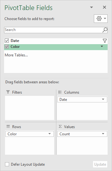
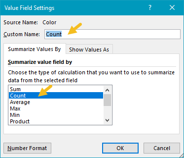
The Color field is configured as a row field, and a value field. In the Values area, the Color field has been renamed “Count” and set to summarize by count:
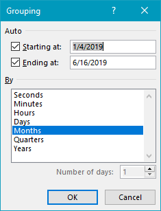
The Date field is grouped by Months only:
To force display of months with no data, the Date field has “Show items with no data” enabled:
<img loading=“lazy” src=“https://exceljet.net/sites/default/files/images/pivot/inline/pivot%20table%20months%20with%20no%20data%20date%20field%20settings.png" onerror=“this.onerror=null;this.src=‘https://blogger.googleusercontent.com/img/a/AVvXsEhe7F7TRXHtjiKvHb5vS7DmnxvpHiDyoYyYvm1nHB3Qp2_w3BnM6A2eq4v7FYxCC9bfZt3a9vIMtAYEKUiaDQbHMg-ViyGmRIj39MLp0bGFfgfYw1Dc9q_H-T0wiTm3l0Uq42dETrN9eC8aGJ9_IORZsxST1AcLR7np1koOfcc7tnHa4S8Mwz_xD9d0=s16000';" alt=“Check “Show items with no data” for Date field - 9”>
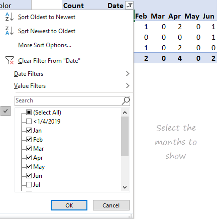
Date filter is set to display only desired months:
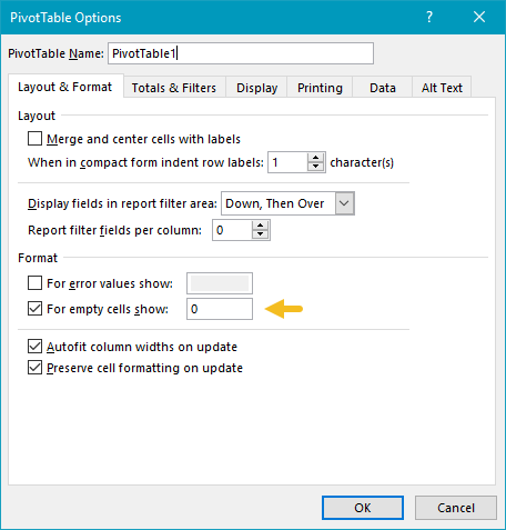
To force the pivot table to display zero when items have no data, a zero is entered in general pivot table options:
Steps
- Create a pivot table
- Add Color field the Rows area (optional)
- Add Date field to Columns area Group Date by Months Set Date to show items with no data in field settings Filter to show only desired months
- Add Color field to Values area Rename to “Count” (optional) Change value field settings to show count if needed
- Set pivot table options to use zero for empty cells
Notes
- Any non-blank field in the data can be used in the Values area to get a count.
- When a text field is added as a Value field, Excel will display a count automatically.
