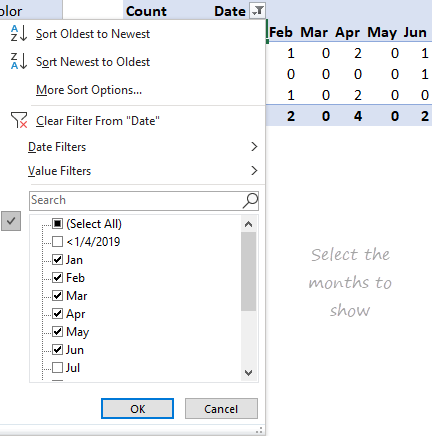
By default, a pivot table shows only data items that have data. When a pivot table is set up to show months, this means that months can “disappear” if the source data does not contain data in that month. In the example shown, a pivot table is used to count the rows by color. There is no data in the months of March and May, so normally these columns would not appear. However, the pivot table shown in the example has been configured to force the display all months between January and June.
Fields
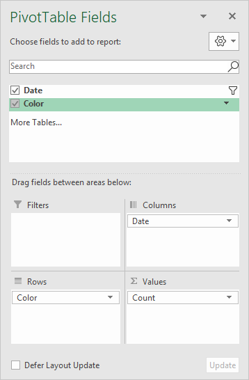
The pivot table shown is based on two fields: Date and Color:
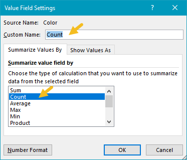
The Color field is configured as a row field, and a value field. In the Values area, the Color field has been renamed “Count” and set to summarize by count:
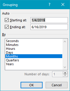
The Date field is grouped by Months only:
To force display of months with no data, the Date field has “Show items with no data” enabled:
<img loading=“lazy” src=“https://exceljet.net/sites/default/files/images/pivot/inline/pivot%20table%20months%20with%20no%20data%20date%20field%20settings.png" onerror=“this.onerror=null;this.src=‘https://blogger.googleusercontent.com/img/a/AVvXsEhe7F7TRXHtjiKvHb5vS7DmnxvpHiDyoYyYvm1nHB3Qp2_w3BnM6A2eq4v7FYxCC9bfZt3a9vIMtAYEKUiaDQbHMg-ViyGmRIj39MLp0bGFfgfYw1Dc9q_H-T0wiTm3l0Uq42dETrN9eC8aGJ9_IORZsxST1AcLR7np1koOfcc7tnHa4S8Mwz_xD9d0=s16000';" alt=“Check “Show items with no data” for Date field - 4”>
Date filter is set to display only desired months:
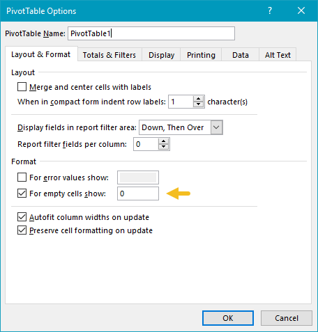
To force the pivot table to display zero when items have no data, a zero is entered in general pivot table options:
Steps
- Create a pivot table
- Add Color field the Rows area (optional)
- Add Date field to Columns area Group Date by Months Set Date to show items with no data in field settings Filter to show only desired months
- Add Color field to Values area Rename to “Count” (optional) Change value field settings to show count if needed
- Set pivot table options to use zero for empty cells
Notes
- Any non-blank field in the data can be used in the Values area to get a count.
- When a text field is added as a Value field, Excel will display a count automatically.
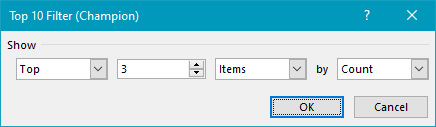
To list and count the most frequently occurring values in a set of data, you can use a pivot table. In the example shown, the pivot table displays the top Wimbledon men’s singles champions since 1968 . The data itself does not have a count, so we use a pivot table to generate a count, and then filter on this value. The result is a pivot table that shows the top 3 players, sorted in descending order by how often they appear in the list.
Note: When there are ties in top or bottom values, Excel will display all tied records. In the example shown, the pivot table is filtered on top 3 but displays 4 players, because Borg and Djokovic are tied for third place.
Data
The source data contains three fields: Year, Country, and Champion. This data is contained in an Excel Table starting in cell B4. Excel Tables are dynamic and will automatically expand and contract as values are added or removed. This allows the Pivot Table to always show the latest list of unique values (after refresh).
Fields
In the pivot table itself, only the Champion field is used, once as a Row field, and once as a Value field (renamed “Count”).
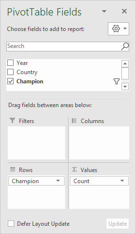
In the Values area, Champion is renamed “Count”. Because Champion is a text field, the value is summarized by Sum.
In the Rows area, the Champion field has a value filter applied, to show only the top 3 players by count (i.e. the number of times each player appears in the list):
In addition, the Champions field is sorted by Count, largest to smallest:

Steps
- Convert data to an Excel Table (optional)
- Create a Pivot Table (Insert > Pivot Table)
- Add the Champion field to the Rows area Rename to “Count” Filter on top 3 by count Sort largest to smallest (Z-A)
- Disable Grand Totals for rows and columns
- Change layout to Tabular (optional)
- When data is updated, Refresh the pivot Table for the latest list
