One of the quirks of pivot tables is that they may hold on to items that have been previously removed from the source data, even after refreshing the data. You may see these deleted “ghost” items when filtering a pivot table. In the example shown, the source data originally contained three colors: red, blue, and green. At some point after the pivot table was created, the color Green disappeared from the source data. However, “Green” still appears when filtering by color in the pivot table.
Remove deleted items from a pivot table
In Excel 2019, and Excel 365 , you can remove deleted items by changing a pivot table setting:
- Right-click the pivot, select PivotTable Options
- Switch to the Data tab
- Under “Retain items deleted from the data source”, select None:
- Click OK to exit
- Refresh the data
- Check the filter drop-down:
Set option for all new pivot tables
To change this setting for all new pivot tables:
- File > Options
- Data > Data options > Edit Default Layout
- Pivot Table Options button > Data
- Set options as above.
Older Excel versions
Older versions of Excel don’t have the setting shown above. To remove deleted items, you’ll need to use a macro. Debra Dalgleish has a detailed explanation here .
Pivot tables have a built-in feature to calculate running totals. In the example shown, a pivot table is used group data by month and show both the monthly total and running total over a 6-month period.
Fields
The source data contains three fields: Date , Sales , and Color . Only two fields are used to create the pivot table: Date and Sales .
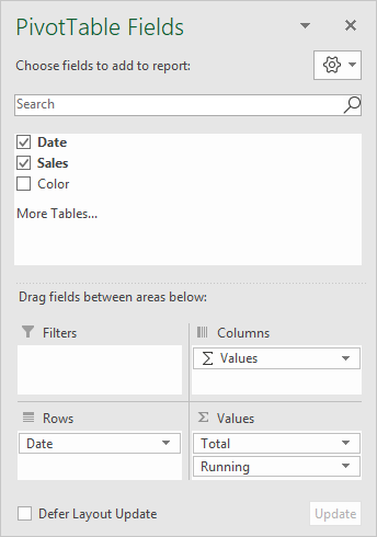
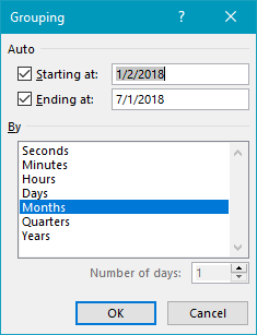
The Date field has been added as a Row field, then grouped by Months:
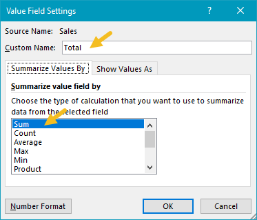
The Sales field has been added twice as a Value field. The first instance is a simple sum, and has been renamed “Total”:
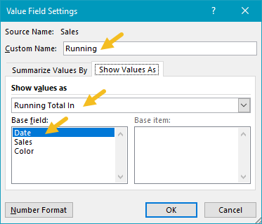
The second instance is renamed “Running” and set to calculate a running total based on the Date field:
Helper column alternative
This example uses automatic date grouping. As an alternative, you can add a helper column to the source data, and use a formula to extract the month name . Then add the Month field to the pivot table directly.
Steps to make this pivot table
- Create a pivot table
- Add Date field to Rows area, group by Months
- Add Sales field Values area Rename to “Total” Summarize by Sum
- Add Sales field Values area Rename to “Running” Show value as running total Set base field to Date
