Pivot tables have a built-in feature to calculate running totals. In the example shown, a pivot table is used group data by month and show both the monthly total and running total over a 6-month period.
Fields
The source data contains three fields: Date , Sales , and Color . Only two fields are used to create the pivot table: Date and Sales .
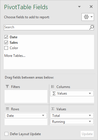
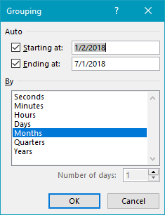
The Date field has been added as a Row field, then grouped by Months:
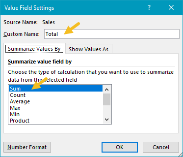
The Sales field has been added twice as a Value field. The first instance is a simple sum, and has been renamed “Total”:
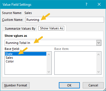
The second instance is renamed “Running” and set to calculate a running total based on the Date field:
Helper column alternative
This example uses automatic date grouping. As an alternative, you can add a helper column to the source data, and use a formula to extract the month name . Then add the Month field to the pivot table directly.
Steps to make this pivot table
- Create a pivot table
- Add Date field to Rows area, group by Months
- Add Sales field Values area Rename to “Total” Summarize by Sum
- Add Sales field Values area Rename to “Running” Show value as running total Set base field to Date
Pivot tables make it easy to count values in a data set. One way this feature can be used is to display duplicates. In the example shown, a pivot table is used to show duplicate cities in an Excel Table that contains more than 250 rows.
Fields
The data contains 263 rows, each with a City and Country. The pivot table shown is based on just one field: City, which has been added as both a Row field and a Value field:

In the Values area, the City field has been renamed “Count” and set to summarize by count :

In the Rows area, the City field is filtered to show only cities where the count is greater than 1:

In addition, the City field is set to sort by count in descending order:

Steps
- Create a pivot table
- Add the City field to the rows area
- Add the City field to the values area Summarize by count Rename “Count” Filter on Cities where count > 1 Sort in descending order by count
