You can use a pivot table to display the top or bottom values in a set of data. In the example shown, one pivot table is used to show the top 3 scores in a set of data, and another pivot table is used to show the bottom 3 values in the same set of data. Because one pivot table was cloned from another, they share the same pivot cache, and both will update when either pivot is refreshed.
How to make this pivot table
- Create a new pivot table on the same worksheet
- Add the Name field to the Rows area
- Add the Score field to the Values area
- Rename the Score field from “Sum of Score” to “Score " (note trailing space)
- Filter values to show “Top 3 items by Score”
- Set sort to “Descending by Score”
- Copy entire pivot table and paste at cell I4
- Filter values to show “Bottom 3 items by Score”
- Set sort to “Ascending by Score”
- Disable grand totals if desired
To build a pivot table to summarize data by month, you can use the date grouping feature. In the example shown, the pivot table is uses the Date field to automatically group sales data by month.
Pivot Table Fields
In the pivot table shown, there are three fields, Name, Date, and Sales. Name is a Row field, Date is a Column field grouped by month, and Sales is a Value field with the Accounting number format applied.
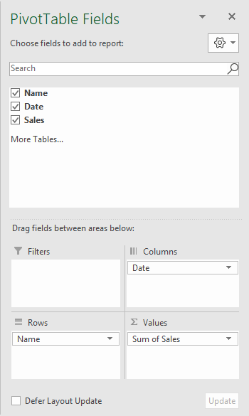
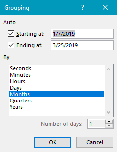
The Date field is grouped by Month, by right-clicking on a date value and selecting “Group”.
Steps
- Create a pivot table
- Add fields to Row, Column, and Value areas
- Right-click a Date field value and set “Group” setting as needed
Notes
- Number formatting doesn’t work on grouped dates because they behave like text.
- As a workaround, add helper column (s) to source data for Year and Month, then use those fields for grouping instead.
