Pivot tables are an easy way to quickly average unique values in a data set, and can easily be adapted to perform a two-way average. In the example shown above, a pivot table is used to average Ratings for unique combinations of Age and Gender, based on data in the range B5:D16, defined as an Excel Table .
Fields
The pivot table shown is based on three fields: Age, Gender, and Rating. The Age field is added as a Row field, and the Gender field is added as a Column field. The Rating field is added as a Value field:
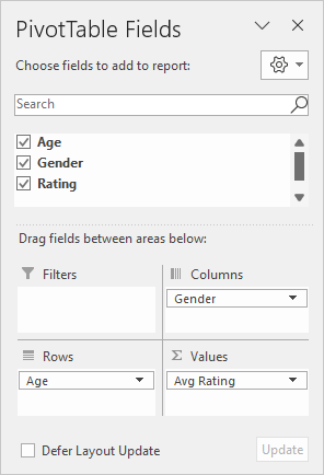
The Rating field in the Values area is renamed to “Avg Rating” and configured to Average:
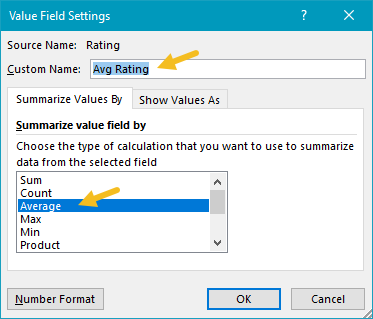
The custom name can be anything except an existing source field name (i.e. not “Age”, “Gender”, or “Rating”).
Steps
- Define data as an Excel Table (optional)
- Create a pivot table based on a table or data
- Add the Age field to the Rows area
- Add the Gender field to the Columns area
- Add the Rating field to the Values area
- Change Rating calculation to Average
- Rename Rating field (optional)
Notes
- When a numeric field is added as a Value field, Excel the field is automatically summed.
Pivot tables are an easy way to quickly count unique values in a data set, and can easily be adapted to perform a two-way count. In the example shown above, a pivot table is used to count unique combinations of color and size, based on data in the range B5:D16, defined as an Excel Table .
Fields
The pivot table shown is based on three fields: Color, Size, and Qty. The Color field is configured as a Rows field, and the Size field is configured as a Columns field. The Color field is also configured as a Value field.

The Color field is configured to summarize by count in the Values area:

Because the colors are text values, the pivot table automatically performs a count instead of a sum. You are free to rename “Count of Color” as you like.
Steps
- Define data as an Excel Table (optional)
- Create a pivot table based on table (or data)
- Add Color field to the Rows area
- Add Size field to the Columns area
- Add Colors field to the Values area
Notes
- Any non-blank field in the data can be used in the Values area to get a count.
- When a text field is added as a Value field, Excel will display a count automatically.
