Explanation
In the worksheet shown, column B contains 12 dates. The goal is to calculate the previous working day before each date, taking into account weekends (Saturday and Sunday) and the holidays listed in column F. The formula should automatically skip weekends and any dates considered non-working days.
WORKDAY function
The WORKDAY function takes a date and returns the “next” working day n days in the future or the past . You can use the WORKDAY function to calculate things like project start dates, delivery dates, and finish dates that need to take into account working and non-working days. The generic syntax for WORKDAY looks like this:
=WORKDAY(start_date,days,[holidays])
Where days is a number (n) and holidays is an optional range that contains non-working dates. For this problem we want the previous working day, so we provide -1 for days . The formula in D5, copied down, looks like this:
=WORKDAY(B5,1,holidays)
Where holidays is the named range F5:F15, which contains dates that should be excluded . The WORKDAY function is fully automatic. Given a valid date, it will move forward or backward by n days, skipping weekends and holidays, until it lands on a working day. Notice we provide a negative 1 for days to move backward. Also, note that we have provided the holidays argument as the named range “holidays” (F5:F15). Without a named range, use an absolute references like $F$5:$F$15:
=WORKDAY(B5,-1,$F$5:$F$15)
As the formula is copied down, it returns the previous business day before the starting date in column B. Saturdays and Sundays are automatically skipped, as well as dates that appear in the range F5:F15.
Current or previous workday
A common scenario in business is that you have a list of dates that may or may not be working days, and you want to shift dates that are not working days back to the previous working day and leave the other dates alone. In that case, you can adjust the formula as follows:
=WORKDAY(B5+1,-1,holidays)
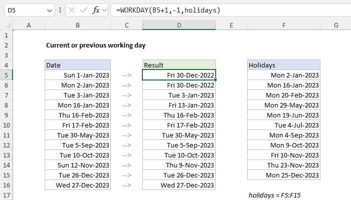
In this version of the formula, we add 1 day to the date inside the WORKDAY function. WORKDAY then moves back one day to the original date and checks the result. If the original date is a working day, WORKDAY returns it. Otherwise, WORKDAY will continue moving back one day at a time until it finds a valid workday, skipping weekends and holidays along the way. You can see the result of this alternate formula in the screen above. For a practical example of this approach, see this formula for semimonthly pay dates .
Custom weekends
The WORKDAY function defines a weekend as Saturday and Sunday only. If you need to provide a more custom workday schedule, switch to the WORKDAY.INTL function instead. For example, to calculate the previous working day in a 4-day workweek where weekends are Friday, Saturday, and Sunday, you can use WORKDAY.INTL like this:
=WORKDAY.INTL(B5,-1,"0000111",holidays)
WORKDAY.INTL includes an optional argument called weekend that can be provided as a string of 1s and 0s like “0000111”. In this scheme, the week begins on Monday and there are 7 characters one for each day of the week. A 1 indicates a weekend and 0 indicates a workday. For more details, see How to use the WORKDAY.INTL function .
Explanation
In this example, the goal is to use a formula to remove the time value from a timestamp that includes both the date and time. To solve this problem, it’s important to understand that Excel handles dates and time using a scheme in which dates are large serial numbers and times are fractional values . For example, June 1, 2000 12:00 PM is represented in Excel as the number 36678.5, where 36678 is the date portion and .5 is the time portion. This means the main task in this problem is to remove the decimal portion of the number.
Note: This example requires valid dates. If you have dates in Excel that don’t seem to be dates, try formatting the cells with the General format . If the date is really a date, you’ll see a number. If the date is being treated as text in Excel, nothing will change.
Number format option
Before permanently removing the time portion of a date, it’s important to understand that you have the option of suppressing the time with a number format . For example, to display “06-Jun-2000 12:00 PM” as “06-Jun-2000”, you can apply a number format like this:
dd-mmm-yyyy
This number format will show the date but hide the time. However, the time will still be there. If the goal is to permanently remove the time portion of a timestamp, see the formulas below.
Note: Excel’s date formats are flexible and can be customized in many ways .
INT function
The INT function returns the integer part of a decimal number by rounding the number down to the integer. For example:
=INT(10.8) // returns 10
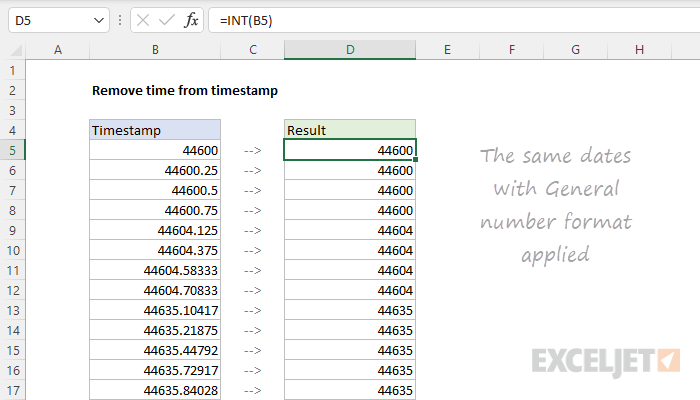
Accordingly, if you have dates in Excel that include time, you can use the INT function to remove the time portion of the date. For example, assuming cell A1 contains the date and time, June 1, 2000 12:00 PM (equivalent to the number 36678.5), the formula below returns just the date portion (36678):
=INT(A1)
=INT(36678.5)
=36678
Notice that the time portion of the date (the fractional part) is permanently discarded, leaving only the integer value. The screen below shows the original dates with the General number format applied, so you can see what is really happening with all of the dates:
Note: to see results formatted as a date, be sure to apply a date number format . Make sure you use a date format that does not include a time . Otherwise, you’ll see the time displayed as 12:00 AM even though the time value has been removed. This is normal Excel behavior.
TRUNC function
You will sometimes see the TRUNC function used as an alternative to the INT function. Like the INT function, the TRUNC function also removes the decimal portion of a number. Unlike INT, the TRUNC function doesn’t round, it truncates a number. In practice, the result is the same with timestamps:
=TRUNC(A1)
=TRUNC(36678.5)
=36678
Although the TRUNC function and the INT function behave differently with negative numbers , this difference doesn’t affect dates which are by definition positive numbers in Excel. So, in practice, there is no difference between INT and TRUNC in this particular case.
Explanation
In the worksheet shown, column B contains 12 dates. The goal is to calculate the next working day after each date, taking into account weekends (Saturday and Sunday) and the holidays listed in column F. In other words, the formula should automatically skip weekends and any dates defined as non-working days.
WORKDAY function
The WORKDAY function takes a date and returns the next working day n days in the future or past. You can use WORKDAY to calculate things like ship dates, delivery dates, and completion dates that need to take into account working and non-working days. The generic syntax for WORKDAY looks like this:
=WORKDAY(start_date,days,[holidays])
Where days is a number (n) and holidays is an optional range that contains non-working dates. For this problem, we want the next working day, so we provide 1 for days . The formula in D5, copied down, looks like this:
=WORKDAY(B5,1,holidays)
Where holidays is the named range F5:F15, which contains days that should be excluded. The WORKDAY function is fully automatic. Given a valid date, it will add days to the date, skipping weekends and holidays. Named ranges behave like absolute references by default, so the range will not change as the formula is copied down. Without a named range, you will need to lock the reference like this:
=WORKDAY(B5,1,$F$5:$F$15)
As the formula is copied down, it returns the next business day after the starting date in column B. Saturdays and Sundays are automatically skipped, as well as any dates that appear in the range F5:F15.
Current date or next workday
There may be situations where you want to return the current date when it’s a working day or the next working date if not. To do this, you can adjust the formula like so:
=WORKDAY(B5-1,1,holidays)
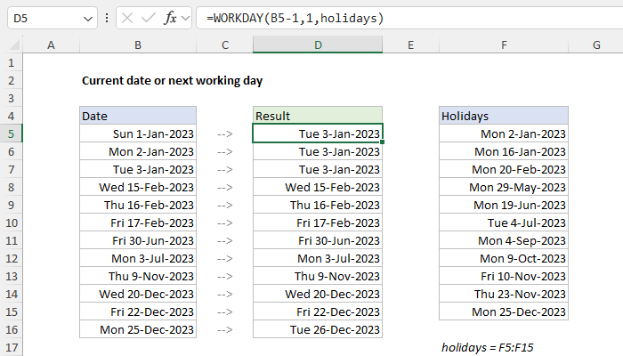
Here, we first subtract 1 day from the date inside the WORKDAY function, then feed that date to WORKDAY as the start_date . WORKDAY then moves forward one day to the original date and checks the result. If the original date is a working day, WORKDAY returns the date unchanged. Otherwise, WORKDAY will continue to move forward one day at a time, skipping weekends and holidays along the way, until it finds a valid workday. You can see the result in the worksheet above.
Custom weekends
The WORKDAY function defines a weekend as Saturday and Sunday only. If you need more flexibility on which days of the week are considered weekends or working days, use the WORKDAY.INTL function instead. For example, to calculate the next working day for this example with a standard work week of Monday-Thursday, where weekend days are Friday, Saturday, and Sunday, you can use WORKDAY.INTL like this:
=WORKDAY.INTL(B5,1,"0000111",holidays)
WORKDAY.INTL includes an extra argument called weekend that can be provided as a string of 1s and 0s like “0000111”. In this scheme, a 1 indicates a weekend and a 0 indicates a workday. For more details, see How to use the WORKDAY.INTL function .
Explanation
Working from the inside out, EDATE first calculates a date 6 months in the future. In the example shown, that date is December 24, 2015.
Next, the formula subtracts 1 day to get December 23, 2015, and the result goes into the WORKDAY function as the start date, with days = 1, and the range B9:B11 provided for holidays.
WORKDAY then calculates the next business day one day in the future, taking into account holidays and weekends.
If you need more flexibility with weekends, you can use WORKDAY.INTL.
