Purpose
Return value
Syntax
=PROPER(text)
- text - The text that should be converted to proper case.
Using the PROPER function
The PROPER function capitalizes each word in a given text string. PROPER function takes just one argument, text , which can be a text value or cell reference. PROPER first lowercases any uppercase letters, then capitalizes each word in the provided text string. Numbers, punctuation, and spaces are not affected. PROPER will convert numbers to text with number formatting removed.
Examples
=PROPER("apple") // returns "Apple"
=PROPER("APPLE") // returns "Apple"
Numbers or punctuation characters inside a text string are unaffected:
=PROPER("XYY-020-kwp") // returns "Xyy-020-Kwp"
If a numeric value is given to PROPER, number formatting is removed. For example, if cell A1 contains the date June 26, 2021, date formatting will be lost and PROPER will return a date serial number as text:
=PROPER(A1) // returns "44373"
Related functions
Use the LOWER function to convert text to lowercase, use the UPPER function to convert text to uppercase, and use the PROPER function to capitalize the words in a text string.
Capitalizing the first word only
One limitation of the PROPER function is that it will capitalize all words in a text string . If you only want to capitalize the first word (i.e. capitalize the first word in a sentence) while leaving other characters unchanged, you can use a custom formula like this:
=REPLACE(A1,1,1,UPPER(LEFT(A1)))
See this page for a full explanation .
Notes
- Use PROPER to capitalize each word in a given string.
- All words in a text string are capitalized.
- Numbers and punctuation characters are not affected.
- Number formatting is removed from standalone numeric values.
Purpose
Return value
Syntax
=REPLACE(old_text,start_num,num_chars,new_text)
- old_text - The text to replace.
- start_num - The starting location in the text to search.
- num_chars - The number of characters to replace.
- new_text - The text to replace old_text with.
Using the REPLACE function
The REPLACE function replaces text at a specific location inside a text string. The location of the text to replace is given as a number representing the first character to replace, along with a character count to indicate how many characters to replace. Unlike SUBSTITUTE , which replaces text by matching content, REPLACE works by position and character count . REPLACE is ideal in cases where the text to replace can’t easily be matched, but the location is predictable.
Key features
- Works by position, not by matching text content
- Is not case-sensitive and does not support wildcards
- Useful when the text to replace has many variations
- Will accept an empty string ("") to remove text completely
- Works in all versions of Excel
You can’t use the REPLACE function by itself to “find and replace” text — it works at a more granular level and swaps text based on position only . For basic find and replace tasks, see the SUBSTITUTE function . For true pattern matching, see the REGEXREPLACE function (Excel 365).
- Example #1 - Basic usage
- Example #2 - Replace different text at same location
- Example #3 - Change first letter
- Example #4 - Remove first characters
- Example #5 - Conditionally remove text
- Example #6 - Capitalized first letter
- Example #7 - Mask credit card numbers
- Related functions
Example #1 - Basic usage
REPLACE function takes four separate arguments in a generic syntax like this:
=REPLACE(old_text,start_num,num_chars,new_text)
The first argument, old_text , is the text string to be processed. The second argument, start_num , specifies the numeric position where replacement should begin. The third argument, num_chars , indicates how many characters to replace. The final argument, new_text , provides the replacement text. You can see how these arguments work in the formulas below:
=REPLACE("C:\docs",1,1,"D") // returns "D:\docs"
=REPLACE("ABC123",4,3,"456") // returns "ABC456"
=REPLACE("XYZ",1,1,"") // returns "YZ"
=REPLACE("www.google.com",1,4,"") // returns "google.com"
- Replace “C” at the start of the path with “D”.
- Replace 3 characters starting at the 4th character (“123” to “456”).
- Replace the “X” at the start with nothing (“X” to “”).
- Remove the first 4 characters (“www.” to “”)
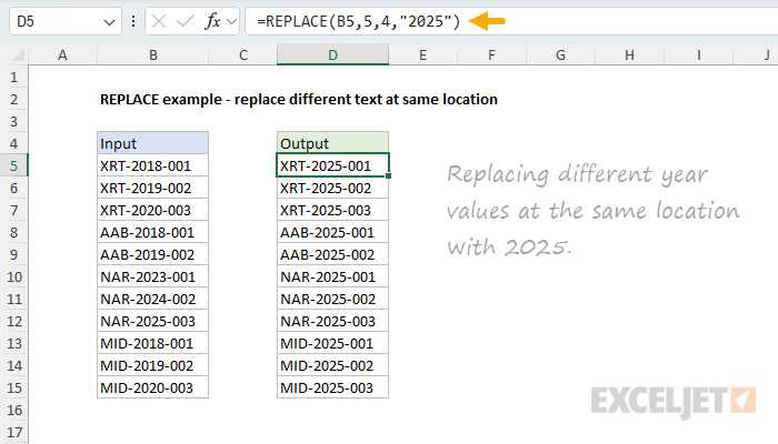
Example #2 - Replace different text at same location
In the example below, the goal is to replace the year values in the middle of the text strings in column B with the year 2025. This is a scenario where the REPLACE function shines. Instead of matching the various year values (as with a function like SUBSTITUTE), we can simply tell replace to replace 4 characters starting at character 5. The formula in cell D5. copied down, looks like this:
=REPLACE(B5,5,4,"2025")
Example #3 - Change first letter
In the worksheet below, the goal is to change the first letter of each path in column B to the letter “Z”. This is another good use case for the REPLACE function because the text we want to change is always fixed at character one, even though it is different in each case. The formula in D5 copied down is:
=REPLACE(B5,1,1,"Z")
<img loading=“lazy” src=“https://exceljet.net/sites/default/files/styles/original_with_watermark/public/images/functions/inline/replace_example_-_change_first_letter.png" onerror=“this.onerror=null;this.src=‘https://blogger.googleusercontent.com/img/a/AVvXsEhe7F7TRXHtjiKvHb5vS7DmnxvpHiDyoYyYvm1nHB3Qp2_w3BnM6A2eq4v7FYxCC9bfZt3a9vIMtAYEKUiaDQbHMg-ViyGmRIj39MLp0bGFfgfYw1Dc9q_H-T0wiTm3l0Uq42dETrN9eC8aGJ9_IORZsxST1AcLR7np1koOfcc7tnHa4S8Mwz_xD9d0=s16000';" alt=“REPLACE example - change first letter in each path to “Z” - 2”>
Notice this is a spill range example. Because we give the REPLACE function 12 values in the range B5:B16 for old_text , it returns 12 results that spill into the range D5:D16.
Example #4 - Remove first characters
The REPLACE function can be used to remove text by providing an empty string (””) for the new_text argument. In the example below, the goal is to strip the “www.” from each domain name in column B. The formula in cell D5, copied down, looks like this:
=REPLACE(B5,1,4,"")
<img loading=“lazy” src=“https://exceljet.net/sites/default/files/styles/original_with_watermark/public/images/functions/inline/replace_example_-_remove_first_characters.png" onerror=“this.onerror=null;this.src=‘https://blogger.googleusercontent.com/img/a/AVvXsEhe7F7TRXHtjiKvHb5vS7DmnxvpHiDyoYyYvm1nHB3Qp2_w3BnM6A2eq4v7FYxCC9bfZt3a9vIMtAYEKUiaDQbHMg-ViyGmRIj39MLp0bGFfgfYw1Dc9q_H-T0wiTm3l0Uq42dETrN9eC8aGJ9_IORZsxST1AcLR7np1koOfcc7tnHa4S8Mwz_xD9d0=s16000';" alt=“REPLACE example - remove “www.” from each domain name - 3”>
Notice we use 1 for start_num and 4 for num_chars , since the text string “www.” contains 4 characters and always starts at character 1. You may need to change these inputs depending on your use case.
Example #5 - Conditionally remove text
In the example below, we have the same problem as above, except the www isn’t always present. This means we need to check for the presence of these characters before we remove them. Otherwise, we’ll remove characters we don’t want to remove. There are a variety of ways to do this in Excel. In the formula below, we’re using the LEFT function inside the IF function to perform this check. The formula in cell D5 looks like this:
=IF(LEFT(B5,4)="www.",REPLACE(B5,1,4,""),B5)
<img loading=“lazy” src=“https://exceljet.net/sites/default/files/styles/original_with_watermark/public/images/functions/inline/replace_example_-_conditionally_remove_text.png" onerror=“this.onerror=null;this.src=‘https://blogger.googleusercontent.com/img/a/AVvXsEhe7F7TRXHtjiKvHb5vS7DmnxvpHiDyoYyYvm1nHB3Qp2_w3BnM6A2eq4v7FYxCC9bfZt3a9vIMtAYEKUiaDQbHMg-ViyGmRIj39MLp0bGFfgfYw1Dc9q_H-T0wiTm3l0Uq42dETrN9eC8aGJ9_IORZsxST1AcLR7np1koOfcc7tnHa4S8Mwz_xD9d0=s16000';" alt=“REPLACE example - remove “www.” only when it actually exists! - 4”>
Note: In a current version of Excel, you can also use the TEXTAFTER function to solve this problem and the previous problem.
Example #6 - Capitalized first letter
It is possible to combine the REPLACE function with other functions that do more sophisticated text manipulation. For example, in the worksheet below, we use the REPLACE function together with the UPPER and LEFT functions to capitalize the text strings in column B. The formula in cell D5 copied down is:
=REPLACE(B5,1,1,UPPER(LEFT(B5)))
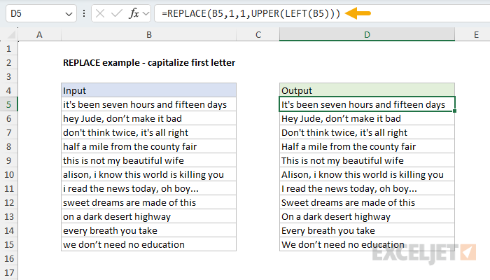
This page explains this formula in more detail and provides some alternatives.
Mask credit card numbers
In the worksheet below, the goal is to mask credit card numbers so that only the last four digits are visible. This is accomplished by combining the REPLACE function with the LEN and REPT functions in a clever formula like this in cell D5:
=REPLACE(B5,1,LEN(B5)-4,REPT("*",LEN(B5)-4))
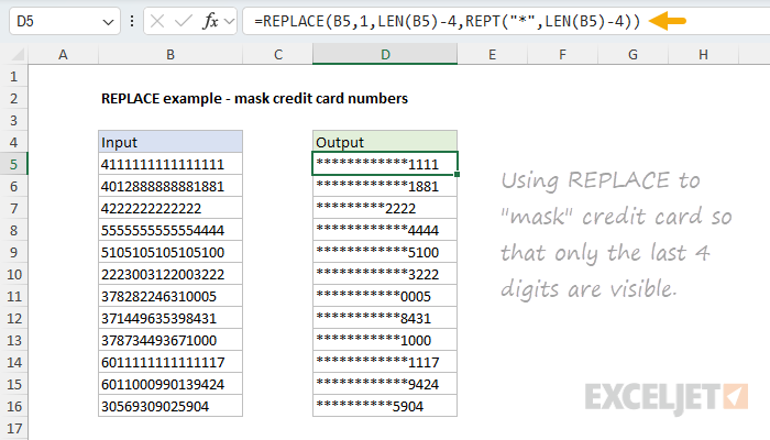
The start number is always 1. To work out the number of characters to replace, we calculate the length of the text string, then subtract 4 to account for the numbers we don’t want to replace: LEN(B5)-4 . To generate the replacement text, we use the REPT function configured to repeat an asterisk () once for each number we are replacing, like this: REPT(”",LEN(B5)-4) .
Related functions
Excel contains several functions that can help you find and replace text:
- REPLACE – Replace text by position when you know the starting point.
- FIND / SEARCH – Find the numeric position of text.
- SUBSTITUTE - replace text with simple matching.
- REGEXREPLACE – Pattern‑based find and replace (Excel 365 only).
Notes
- To remove text, use an empty string (””) for new_text .
- REPLACE returns #VALUE is start_num or num_chars is not a positive number.
- REPLACE works on numbers, but the result is text.
