Explanation
In this example, the goal is to return a random group (“A”, “B”, or “C”) at each new row. The simplest way to do this is to use the RANDBETWEEN function with the CHOOSE function. In the current version of Excel, it is also possible to generate all random groups in one step with the RANDARRAY function. Both approaches are explained below.
The CHOOSE function
The CHOOSE function returns a value from a list of values using an index number. The index number is provided as the first argument, and the values to be selected follow. For example, if we have a list of three colors (“red”, “blue”, and “green”), we can configure CHOOSE to return each color in turn with the following formulas:
CHOOSE(1,"red","blue","green") // returns "red"
CHOOSE(2,"red","blue","green") // returns "blue"
CHOOSE(3,"red","blue","green") // returns "green"
Notice that CHOOSE uses the index number to select the “nth” value from the list of values. The values can be customized in any way you like and the only requirement is that the index number be valid for the number of values provided. Of course, in this example, we don’t want to hardcode an index number into CHOOSE, we want a random index number. For this, we can use the RANDBETWEEN function.
The RANDBETWEEN function
The RANDBETWEEN function generates a random number between two integers, provided as the bottom and the top . For example, to generate a random number between 1 and 10, you can use RANDBETWEEN like this:
=RANDBETWEEN(1,10) // returns a random number between 1 and 10
When Excel’s calculation engine updates a worksheet, RANDBETWEEN will generate a random number between 1 and 10.
CHOOSE with RANDBETWEEN
The behavior of RANDBETWEEN will work perfectly for this problem. We have three possible groups (“A”,“B”,“C”) so we need a random number between 1 and 3, which we can get like this:
=RANDBETWEEN(1,3) // returns a random number between 1 and 3
The final step is to embed RANDBETWEEN into the CHOOSE function as the index number like this:
=CHOOSE(RANDBETWEEN(1,3),"A","B","C")
This is the formula that appears in cell F5 in the example shown. When the formula is copied down the column, RANDBETWEEN returns a random number between 1 and 3. This number is delivered directly to the CHOOSE function as the index number, and CHOOSE returns the corresponding color as a final result. You can use this approach whenever you need to assign random text values to each row in a data set. Just be sure to adjust the second argument in RANDBETWEEN, top , to match the number of values provided.
Stopping automatic recalculation
Be aware that RANDBETWEEN is a volatile function and will recalculate whenever there is any change to a workbook, or even when a workbook is opened. To force a recalculation, you can press the F9 key. Once you have a set of random assignments, you may want to stop the formula from returning new results. The classic way to do this is to use Paste Special:
- Select all cells that contain the CHOOSE and RANDBETWEEN formula.
- Copy to the clipboard with Control + C.
- Open the Paste Special window with the shortcut Control + Alt + V.
- Select “Values” and click OK:
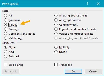
After you press OK, all formulas will be replaced with static values.
Dynamic array formula
In the current version of Excel (Excel 2021 or later) you can use a single dynamic array formula to generate all random values at once. One option is to use the RANDARRAY function with CHOOSE like this:
=CHOOSE(RANDARRAY(ROWS(B5:B104),,1,3,TRUE),"A","B","C")
The core idea of this formula is the same as the original formula above. However, instead of RANDBETWEEN, we use RANDARRAY, which can generate an array of random numbers in one step. To figure out how many random numbers to generate, we use the ROWS function on a range corresponding to the first column of the data. This saves us the step of telling RANDARRAY how many rows we need. In this case, ROWS returns 100, because there are 100 rows in the range B5:B104. Simplifying, we now have:
=CHOOSE(RANDARRAY(100,,1,3,TRUE),"A","B","C")
Next, RANDARRAY generates an array of 100 random numbers between 1 and 3. The result is returned to CHOOSE as the index_num argument, and CHOOSE uses the random numbers to return an array that contains 100 random groups. This array lands in cell F5 and spills into the range F5:F104.
RANDARRAY is a volatile function and will recalculate with each worksheet change.
INDEX alternative
It is also possible to use the INDEX function instead of CHOOSE in a formula like this:
=INDEX({"A","B","C"},RANDBETWEEN(1,3))
Like CHOOSE, INDEX retrieves a value based on an index number. INDEX however accepts the values all at once in the first argument, called array . In the formula above, the values “A”, “B”, and “C” are provided as an array constant to INDEX as the array , and RANDBETWEEN is used as before to generate a random number between 1 and 3. The RANDARRAY version of the formula with INDEX looks like this:
=INDEX({"A","B","C"},RANDARRAY(ROWS(B5:B104),,1,3,TRUE))
One advantage of INDEX is that the array constant can be replaced with a range on the worksheet. In other words, you can enter group names into a range and provide that range to INDEX. The CHOOSE function will not accept a range of values; it requires that values be provided separately.
Note: the formulas on this page will create completely random groups. One result is that the total number of rows assigned to each group will vary. If you need to assign random groups with a fixed size (i.e. randomly assign people to teams of 6), see the example on this page .
Explanation
In this example, the goal is to randomly assign the names in column B to three groups of equal size. The group names are “A”, “B”, and “C”, and these values appear in the named range groups (F5:F7). The solution should automatically count the number of groups to assign and attempt to generate the same count for each group. The worksheet shown contains 18 names, the final result should be that each group includes 6 random names from the list. The article below explains two approaches: (1) a traditional formula that depends on random values in a helper column, which will work in any version of Excel, and (2) a Dynamic Array formula that will return all random groups in one step without a helper column.
The solutions explained here are more complex because we are taking care to place the same number of people in each group when possible. To simply assign random groups without regard to size, see this page .
Basic approach
For both formulas explained below, the basic approach is the same and looks like this:
- Generate random numbers for each row
- Rank the random numbers
- Count groups and calculate the ideal group size
- Divide each rank by the group size
- Round the results up to the nearest whole number
- Use the whole number to fetch a group name with INDEX
The difference below is in the implementation. In older versions of Excel, we need to add a helper column that contains random numbers to the data, then use a formula that ranks each row according to the helper column. In the current version of Excel, we can use a single formula that generates all random numbers at once, and there is no need for a helper column.
Traditional formula
The traditional way to solve this problem in an older version of Excel is to use a helper column populated with random numbers with the RAND function , as seen in the worksheet above. In the worksheet shown, the random numbers appear in the range C5:C22 which is named “randoms” for convenience. To generate a full set of random values in one step, select the range C5:C22 and type =RAND() in the formula bar. Then use the shortcut control + enter to enter the formula in all cells at once.
Note: the RAND function will keep generating random values every time a change is made to the worksheet, so typically you will want to replace the results in column C with actual values using paste special to prevent changes after random values are assigned.
Assigning groups with INDEX
The formula used to assign random groups looks like this:
=INDEX(groups,ROUNDUP(RANK(C5,randoms)/(ROWS(randoms)/COUNTA(groups)),0))
At a high level, this formula uses the INDEX function to assign a group of “A”, “B”, or “C” to each name in the list. The generic pattern looks like this, where n is a number that corresponds to a group:
=INDEX(groups,n)
Because there are three groups total, the value for n needs to be between 1 and 3:
=INDEX(groups,1) // returns "A"
=INDEX(groups,2) // returns "B"
=INDEX(groups,3) // returns "C"
The hard part of the formula is generating a random number (n) for each row that will result in three groups of equal size. This is done in the snippet below, which makes up the bulk of the formula:
ROUNDUP(RANK(C5,randoms)/(ROWS(randoms)/COUNTA(groups)),0)
Working from the inside out, the first step is to assign a numeric rank to each random number with the RANK function :
RANK(C5,randoms)
RANK compares the number in cell C5 to all values in C5:C22 and returns its position relative to the other numbers in the range. The smallest number gets rank 1, the next smallest rank 2, and so on. Because there are 18 numbers in the list, RANK will generate a rank of 1-18. The next part of the formula calculates the optimal size for each group by dividing the total number of rows in the data by the number of groups to assign:
ROWS(randoms)/COUNTA(groups)
The ROWS function returns a count of rows (18), and the COUNTA function returns a count of groups (3). Simplifying, we have:
=ROWS(randoms)/COUNTA(groups)
=18/3
=6
The result is 6, which is the number of names that should be in each of the three groups. Next, the rank of each random number is divided by the number of names per group (6):
rank/6
For example, when a row is ranked 1st, the formula would return a value of 1/6, or 0.1667, when a row has a rank of 6, the formula returns 1/1, or 1, and so on. This is the mechanism by which the formula generates groups of equal size. The final step is to use the ROUNDUP function to round each number up to the next whole number, effectively dividing the ranked individuals into three equally sized groups based on their rank. The result from ROUNDUP is a random number between 1-3 (n) which is then used by INDEX to assign a group.
Dynamic Array formula
In Excel 2021 or later, dynamic array formulas allow a more sophisticated solution with an all-in-one formula that requires no helper columns. In the screen below, the formula in cell C5 is:
=LET(
ct,ROWS(B5:B22),
groups,E5:E7,
size,ct/COUNTA(groups),
randoms,SORTBY(SEQUENCE(ct),RANDARRAY(ct)),
INDEX(groups,ROUNDUP(randoms/size,0)))
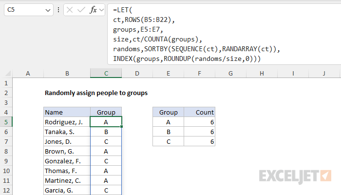
This formula uses the LET function to create named variables within the formula, which reduces complexity and improves readability. In the first part of the formula, four variables are defined as follows:
- ct : The count of names, determined by ROWS(B5:B22) .
- groups : The groups to be assigned in the range E5:E7 .
- size : The size of each group, determined with ct/COUNTA(groups)
- randoms : A sorted list of random numbers created with SORTBY(SEQUENCE(ct), RANDARRAY(ct)) .
The definition of randoms is the most interesting bit:
SORTBY(SEQUENCE(ct),RANDARRAY(ct))
Since ct has been previously defined as 18, the SEQUENCE function creates an array of sequential numbers between 1 and 18. The RANDARRAY function creates an array of random numbers of the same size. Next, the SORTBY function sorts the sequence in the order of the random numbers, effectively shuffling the sequence. The result is the numbers 1 to 18 in a random order.
With the variables above in place, the last line in the formula generates the random groups like this:
INDEX(groups,ROUNDUP(randoms/size,0))
Like the original formula above, the basic pattern of this formula is:
=INDEX(groups,n)
where n is a random number between 1 and 3, corresponding to the three groups. The 18 individual values for n are calculated in one step like this:
ROUNDUP(randoms/size,0)
First, the numbers in randoms are divided by size to get a decimal number corresponding to a group. Then they handed off to the ROUNDUP function which rounds the numbers up to the nearest whole number. The result from ROUNDUP is an array that contains 18 numbers between 1 and 3. This array is returned directly to INDEX as the row_num argument, and INDEX returns the corresponding 18 groups in one step. The final result is that each group contains 6 random names from the list.
Conclusion
Although both formulas explained above work well, the dynamic array formula keeps all operations in a single cell. There is no need for a helper column. In addition, the LET function allows us to define variables that can be reused in the formula without recalculation, which makes the formula easier to read and more efficient. The result is a dynamic and efficient way to assign individuals to random groups of equal size with a single formula.
