Explanation
In this example, the goal is to use a formula to remove the time value from a timestamp that includes both the date and time. To solve this problem, it’s important to understand that Excel handles dates and time using a scheme in which dates are large serial numbers and times are fractional values . For example, June 1, 2000 12:00 PM is represented in Excel as the number 36678.5, where 36678 is the date portion and .5 is the time portion. This means the main task in this problem is to remove the decimal portion of the number.
Note: This example requires valid dates. If you have dates in Excel that don’t seem to be dates, try formatting the cells with the General format . If the date is really a date, you’ll see a number. If the date is being treated as text in Excel, nothing will change.
Number format option
Before permanently removing the time portion of a date, it’s important to understand that you have the option of suppressing the time with a number format . For example, to display “06-Jun-2000 12:00 PM” as “06-Jun-2000”, you can apply a number format like this:
dd-mmm-yyyy
This number format will show the date but hide the time. However, the time will still be there. If the goal is to permanently remove the time portion of a timestamp, see the formulas below.
Note: Excel’s date formats are flexible and can be customized in many ways .
INT function
The INT function returns the integer part of a decimal number by rounding the number down to the integer. For example:
=INT(10.8) // returns 10
Accordingly, if you have dates in Excel that include time, you can use the INT function to remove the time portion of the date. For example, assuming cell A1 contains the date and time, June 1, 2000 12:00 PM (equivalent to the number 36678.5), the formula below returns just the date portion (36678):
=INT(A1)
=INT(36678.5)
=36678
Notice that the time portion of the date (the fractional part) is permanently discarded, leaving only the integer value. The screen below shows the original dates with the General number format applied, so you can see what is really happening with all of the dates:
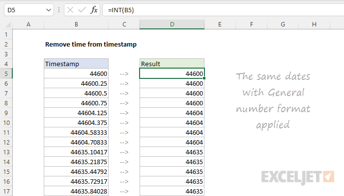
Note: to see results formatted as a date, be sure to apply a date number format . Make sure you use a date format that does not include a time . Otherwise, you’ll see the time displayed as 12:00 AM even though the time value has been removed. This is normal Excel behavior.
TRUNC function
You will sometimes see the TRUNC function used as an alternative to the INT function. Like the INT function, the TRUNC function also removes the decimal portion of a number. Unlike INT, the TRUNC function doesn’t round, it truncates a number. In practice, the result is the same with timestamps:
=TRUNC(A1)
=TRUNC(36678.5)
=36678
Although the TRUNC function and the INT function behave differently with negative numbers , this difference doesn’t affect dates which are by definition positive numbers in Excel. So, in practice, there is no difference between INT and TRUNC in this particular case.
Explanation
The goal of this example is to sum amounts by fiscal year, when the fiscal year begins in July. The first approach is a self-contained formula based on the SUMPRODUCT function. The second method uses SUMIF with column D as a helper column. Either approach will work correctly, and the best option depends on personal preference.
Helper column
To make the example easier to understand and to provide a simple way to use the SUMIF function (see below), column D is set up as a helper column that displays a fiscal year for each row, based on a July start. The formula in cell D5 is:
=YEAR(B5)+(MONTH(B5)>=7)
This formula is explained in detail here .
SUMPRODUCT option
One approach is to use the SUMPRODUCT function together with the YEAR and MONTH functions as seen in the example, where the formula in G5 is:
=SUMPRODUCT(--(YEAR(date)+(MONTH(date)>=7)=F5),amount)
Here, SUMPRODUCT is configured with two arrays. The first array ( array1 ) is set up to filter values based on the fiscal year in column F:
--(YEAR(date)+(MONTH(date)>=7)=F5)
The main part of the formula simply returns the fiscal year for each date in the named range date:
YEAR(date)+(MONTH(date)>=7
Because there are 12 dates in this range, the result is 12 values in an array like this:
{2021;2021;2021;2021;2021;2021;2022;2022;2022;2022;2022;2022}
These are then compared to the year in F5 (2021) and the result is an array with 12 TRUE and FALSE values:
{TRUE;TRUE;TRUE;TRUE;TRUE;TRUE;FALSE;FALSE;FALSE;FALSE;FALSE;FALSE}
A double negative is used to coerce the TRUE and FALSE values to 1s and 0s, which yields:
{1;1;1;1;1;1;0;0;0;0;0;0}
This array is returned directly to the SUMPRODUCT function as array1 :
=SUMPRODUCT({1;1;1;1;1;1;0;0;0;0;0;0},amount)
Array2 is the named range amount (C5:C16) which contains values to sum. SUMPRODUCT multiplies the corresponding items in each array which results in an array like this:
{2350;750;1000;1200;1850;550;0;0;0;0;0;0}
Notice amounts in fiscal year 2022 have been “zeroed out”. Finally, SUMPRODUCT returns the sum of all items in the array, 7700.
SUMIF option
Because each row in the data already contains a calculated value for fiscal year in column D, we can use this column directly in the SUMIF function as a criteria range. With SUMIF, the formula in G5, copied down, is:
=SUMIF(FY,F5,amount)
This is a much simpler formula than the SUMPRODUCT formula above, but it depends on the fiscal year values being part of the data. In contrast, the SUMPRODUCT option is self-contained. We can’t build a similar self-contained formula with SUMIF because of innate limitations of the function . Namely, the cells being evaluated must be a range , they can’t be an array generated by another formula.
