Explanation
The first thing this formula does is check the date in column B against the start date:
=IF(B4>=start
If the date is not greater than the start date, the formula returns zero. If the date is greater than or equal to the start date, the IF function runs this snippet:
(MOD(DATEDIF(start,B4,"m")+n,n)=0)*value
Inside MOD, the DATEDIF function is used to get the number of months between the start date and the date in B4. When the date in B4 equals the start date, DATEDIF returns zero. On the next month, DATEDIF returns 1, and so on.
To this result, we add the value for the named range “n”, which is 3 in the example. This effectively starts the numbering pattern at 3 instead of zero.
The MOD function is used to check each value, with n as the divisor:
MOD(DATEDIF(start,B4,"m")+n,n)=0
If the remainder is zero, we are working with a month that requires a value. Instead of nesting another IF function, we use boolean logic to multiply the result of the expression above by “value”.
In months where there should be a value, MOD returns zero, the expression is TRUE, and value is returned. In other months, MOD returns a non-zero result, the expression is FALSE, and the value is forced to zero.
Explanation
In this example, the goal is to repeat a range of values. This can be done in various ways in Excel, but I think the CHOOSEROWS/ CHOOSECOLS functions are the easiest way to retrieve values from the range for now. Both functions work natively with two-dimensional ranges and can accept a single array of numeric index numbers. The formulas below work in two steps:
- Generate a repeating list of numeric index numbers.
- Use the index numbers to retrieve and repeat values from a range.
Step 1 is based on the formula explained in detail here . Step 2 is based on either the CHOOSEROWS function (to repeat values by row) or the CHOOSECOLS function (to repeat values by column).
Generic formula
The generalized formula for repeating a range into rows looks like this:
=CHOOSEROWS(range,MOD(SEQUENCE(n*x)-1,n)+1)
- range - the range to repeat, or an array constant like {“a”;“b”;“c”}
- n - the number of rows to repeat
- x - the number of times to repeat
Worksheet formula
In the example shown above, we are repeating 3 values {“dog”;“cat”;“fish”} 4 times into 12 rows with this formula in cell D5:
=CHOOSEROWS(B8:B10,MOD(SEQUENCE(3*B5,,0),3)+1)
Step 1: Generate repeating index numbers
The core idea of this approach is to create a repeating sequence of numbers that can be used as indices to retrieve values from a range or array. This is done with the SEQUENCE function and the MOD function here:
MOD(SEQUENCE(3*B5,,0),3)+1
This code creates a single array of repeating numbers. First, SEQUENCE creates an array of 12 sequential numbers starting with zero:
=SEQUENCE(3*4,,0)
=SEQUENCE(12,,0)
={0;1;2;3;4;5;6;7;8;9;10;11}
Next, the MOD function converts the numbers into a repeating sequence:
=MOD({0;1;2;3;4;5;6;7;8;9;10;11},3)+1
={0;1;2;0;1;2;0;1;2;0;1;2}+1
={1;2;3;1;2;3;1;2;3;1;2;3}
The final result is an array like this:
{1;2;3;1;2;3;1;2;3;1;2;3}
Notice that we have repeated the values {1;2;3} four times.
Note: For a more detailed explanation of this part of the formula, which can used standalone, see: Repeat sequence of numbers .
Step 2: Repeat the values
Now that we have an array of repeating numbers, the next step is to use these numbers to extract values in the range B8:B10. To do that, we use the CHOOSEROWS function , which is designed to return specific rows from an array or range. The array from the SEQUENCE and MOD operation described above is delivered directly to CHOOSEROWS as row_num1 :
=CHOOSEROWS(B8:B10,{1;2;3;1;2;3;1;2;3;1;2;3})
Although the signature for CHOOSEROWS suggests that row numbers must be provided separately, an array constant works just fine. The result from CHOOSEROWS is an array with the first three rows of the range B5:B10 repeated 4 times:
{"dog";"cat";"fish";"dog";"cat";"fish";"dog";"cat";"fish";"dog";"cat";"fish"}
This array lands in cell D5 and spills into the range D5:D16.
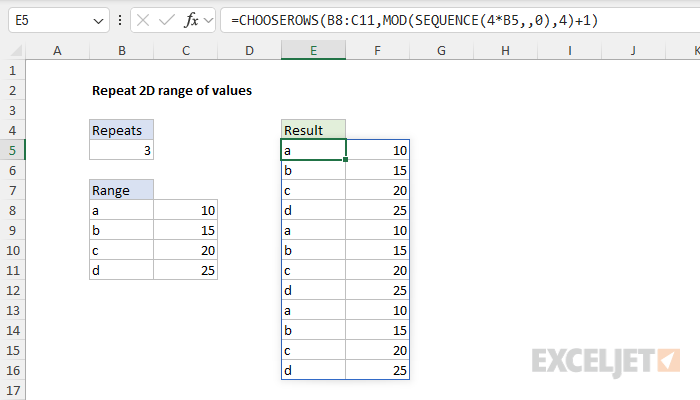
Example with a 2D range
Because we are using the CHOOSEROWS function, we have native support for two-dimensional ranges. In the worksheet below, we repeat the range B8:C11 3 times with this formula in cell E5:
=CHOOSEROWS(B8:C11,MOD(SEQUENCE(4*B5,,0),4)+1)
Repeat range into columns
By switching to CHOOSECOLS, we can repeat a range into columns instead of rows. The CHOOSECOLS function is designed to return specific columns from a range. The generic version of the formula looks like this:
=CHOOSECOLS(range,MOD(SEQUENCE(n*x)-1,n)+1)
In the worksheet below, we use this formula to repeat the range B8:B11 5 times by column:
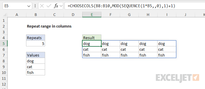
This formula’s operation is the same as the original above, except that we repeat values by column.
