Purpose
Return value
Syntax
=SCAN([initial_value],array,function)
- initial_value - [optional] The initial value of the accumulator. Default is zero.
- array - The array to be scanned.
- function - The function or custom LAMBDA to apply.
Using the SCAN function
The SCAN function applies a custom calculation to each element in a given array and returns an array that contains each intermediate value created during the scan. SCAN can generate running totals, running counts, and other calculations that create intermediate or incremental results. The results returned by SCAN are the value of an “accumulator” at each step in the process.
Like the REDUCE function , SCAN iterates over all elements in an array and performs a calculation on each element while updating the value of an accumulator. However, while REDUCE returns a single value, SCAN returns an array of values.
Key features
- Useful for running totals, running counts, and other “running” results.
- Returns all intermediate values as an array, not just the final result.
- Uses a custom LAMBDA function to apply the calculation.
- Tracks the prior result of a calculation as an “accumulator”.
- Plays nicely with dynamic array formulas (expands with data).
SCAN returns the value of the accumulator when each element in the array is processed. The result is an array of “intermediate” values. To scan an array and return a single aggregated result, see the REDUCE function . To process each element in an array individually and return an array of non-intermediate results, see the MAP function
- LAMBDA structure
- SCAN for a basic running total
- SCAN with abbreviated function syntax
- SCAN with dynamic range
- SCAN for YTD calculations
- SCAN for conditional running totals
- SCAN for running counts
- SCAN with a boolean array
- SCAN for a running count by category
- SCAN with text values
- SCAN for a running MAX
- SCAN to find the longest winning streak
- SCAN for compounded interest
LAMBDA structure
The SCAN function takes three arguments: initial_value , array , and function . Initial_value is the initial seed value to use for the first result. Initial_value is optional and defaults to zero (0). Array is the array or range to scan, and function is typically a LAMBDA function to apply to each value in the array . The structure of the LAMBDA used inside SCAN looks like this:
LAMBDA(a,v,calculation)
The first argument, a , is the accumulator used to store intermediate values. The accumulator begins as the initial_value provided to SCAN and changes as the SCAN function loops over the elements in the array and applies a calculation. The v argument is the value of each element in the array at a given iteration. The calculation is a formula that operates on the accumulator (a) and value (v). The result of the calculation defines the value of the accumulator for the next iteration, and the final result is an array that contains all accumulator values created during the scan. For example, in the formula below, SCAN is used to create a running total of an array with three values:
=SCAN(0,{1,2,3},LAMBDA(a,v,a+v)) // returns {1,3,6}
The initial_value is provided as zero, the array is hard-coded as the array constant {1,2,3}, and the calculation, LAMBDA(a,v,a+v) , simply adds the accumulator and value. The table below shows how the accumulator value changes during each iteration when SCAN processes the array {1,2,3} with an initial value of 0. Notice that the accumulator is updated with the result of the calculation at each iteration.
| Iteration | Value (v) | Accumulator (a) | Calculation | Result |
|---|---|---|---|---|
| Initial | - | 0 | - | - |
| 1 | 1 | 0 | 0 + 1 | 1 |
| 2 | 2 | 1 | 1 + 2 | 3 |
| 3 | 3 | 3 | 3 + 3 | 6 |
The final result returned by SCAN is the array {1,3,6}, which contains all intermediate values calculated during the scan.
The SCAN function always assigns the first argument of LAMBDA to the accumulator (a) and the second argument to the current value (v) from the array. This behavior is built into the function’s design and cannot be changed. The names a and v are arbitrary, used to represent accumulator and value . You can use any names that make sense to you for a given use case.
SCAN for a basic running total
A simple use of SCAN is to create a running total. In the worksheet shown below, we have a list of values in the range B5:B16, and we want to create a running total of the values in the range. The formula in D5 is:
=SCAN(0,B5:B16,LAMBDA(a,v,a+v))
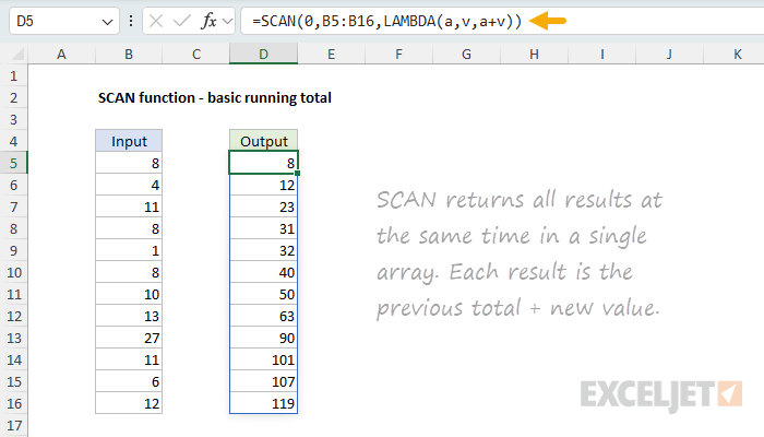
The result is a running sum of values in the range B5:B16. All values are returned at the same time in a single array.
SCAN with abbreviated function syntax
Like other newer dynamic array functions, SCAN supports an abbreviated syntax for the function argument. Using the abbreviated syntax, the formula above can also be written like this:
=SCAN(0,B5:B16,SUM)
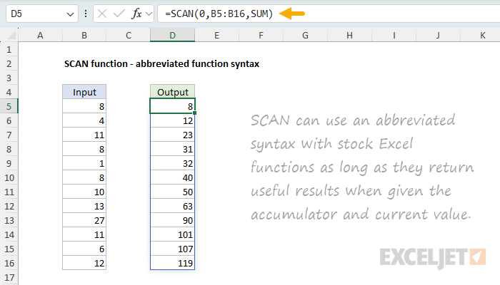
It is not obvious, but SCAN is delivering two values, the accumulator and the value to the SUM function at each loop. The result is a running total. While the abbreviated syntax is handy, note that SCAN’s iterative behavior means that many of Excel’s stock functions won’t return useful results. For example, if we try to use SCAN with COUNT on the data above to create a running count , the result will always be 2:
=SCAN(0,B5:B16,COUNT) // returns {2,2,2,2,2,2,2,2,2,2,2,2}
To illustrate why this is the case, the table below shows how SCAN processes the first 5 values when using COUNT. At each iteration, COUNT returns the number of numeric values it receives. Since it always receives 2 values (the accumulator and the current value), the result is always 2:
| Iteration | Value (v) | Accumulator (a) | Calculation | Result |
|---|---|---|---|---|
| 1 | 8 | 0 | COUNT(0,8) | 2 |
| 2 | 4 | 2 | COUNT(2,4) | 2 |
| 3 | 11 | 2 | COUNT(2,11) | 2 |
| 4 | 8 | 2 | COUNT(2,8) | 2 |
| 5 | 1 | 2 | COUNT(2,1) | 2 |
In general, functions that work well with abbreviated syntax inside of SCAN are those that will operate naturally on two inputs and return useful results (i.e. SUM, MAX, MIN, etc.)
SCAN with a dynamic range
One of SCAN’s key strengths is its ability to work with dynamic arrays. When you give SCAN an array that is dynamically generated, it will automatically adjust the output to match the size of the array as it expands or contracts. You can see an example of this in the screen below, where SCAN has been configured to return a dynamic running total of the values in column B. The formula in cell D5 looks like this:
=SCAN(0,TRIMRANGE(B5:B1000,2),SUM)
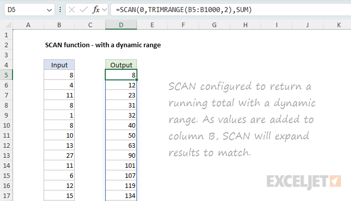
Notice we are using the abbreviated syntax and calling the SUM function directly. The key feature of this formula, which makes the output dynamic, is the use of the TRIMRANGE function to provide the array to SCAN:
TRIMRANGE(B5:B1000,2)
TRIMRANGE will adjust the starting range of B5:B1000 to match the data it contains by removing empty trailing rows. The resulting “trimmed” range is returned directly to SCAN, which returns running totals to match. As a more concise alternative, you can also use the dot operator instead of TRIMRANGE:
=SCAN(0,B5:.B1000,SUM) // dot operator syntax
SCAN also works well with other dynamic ranges in Excel, including values in an Excel Table and spill ranges .
SCAN for YTD calculations
One common use of SCAN is to create a YTD calculation. In the worksheet shown below, we have a list of months in the range B5:B16, and sales numbers in the range C5:C16. We want to create a YTD calculation of the sales numbers in the range. The formula in E5 is:
=SCAN(0,C5:C16,LAMBDA(a,v,a+v))
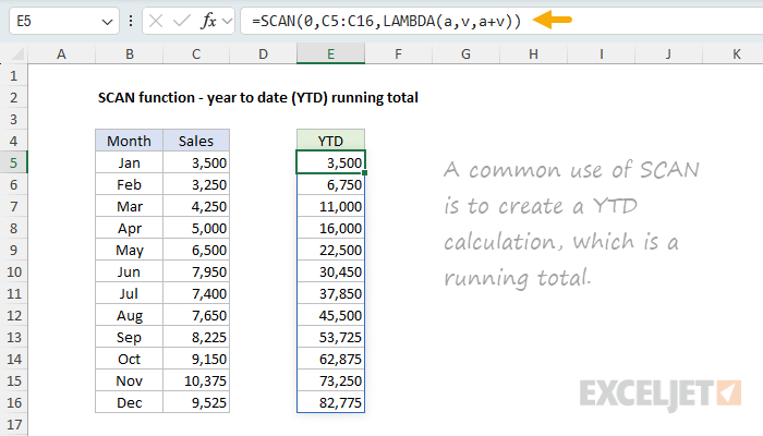
The result is a list of running YTD totals of the values in C5:C16.
SCAN for conditional running totals
Because the calculation applied by SCAN is fully customizable, it is possible to apply conditions. In the worksheet shown below, we have a list of numbers in the range B5:B16, and the goal is to create a running total of the odd numbers in the range. The formula in D5 looks like this:
=SCAN(0,B5:B16,LAMBDA(a,v,IF(ISODD(v),a+v,a)))
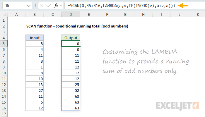
Notice we use the ISODD function inside the IF function to check if the value is odd. If it is, the value is added to the accumulator. If it is not, the accumulator is returned unchanged. The result is a list of running totals of the odd numbers in B5:B16.
SCAN for running counts
SCAN can also be used for running counts. In the worksheet shown below, we have a list of values in the range B5:B16 and the goal is to create a running count of the numbers in the range. The formula in D5 looks like this:
=SCAN(0,B5:B16,LAMBDA(a,v,a+COUNT(v)))
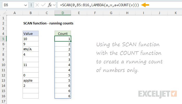
The COUNT function only counts numbers, so it will return 0 for text values, errors, and empty cells. There are 6 numbers in the range, and the final result is an array like this:
{1;2;2;3;3;4;4;5;5;6;6;6}
Notice that the count is only incremented when SCAN encounters a numeric value. Otherwise, the accumulator is returned unchanged. The result is a running count of the numbers in B5:B16. As an alternative to COUNT, you could also use the ISNUMBER function to create a running count of numbers:
=SCAN(0,B5:B16,LAMBDA(a,v,a+ISNUMBER(v)))
In a similar way, you could use ISBLANK to count blanks, ISTEXT to count text values, ISERROR to count errors, and so on.
SCAN with a Boolean array
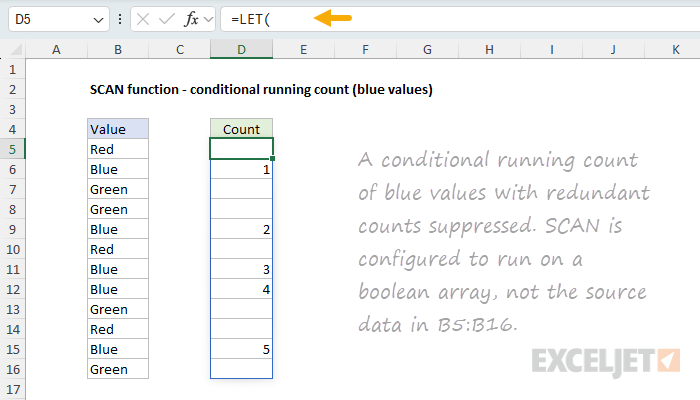
Sometimes it makes sense to perform a Boolean operation on an array and then use the SCAN function to iterate over the result instead of working with the source array. A good example of this is when you want to perform a conditional running count and suppress redundant counts. You can see an example of this in the worksheet below, we have a list of colors in B5:B16, and the goal is to return a running count for the appearance of the color “blue”, but for other colors, we want the result to be blank. The formula in D5 looks like this:
=LET(
    hits,B5:B16="Blue",
    counts,SCAN(0,hits,LAMBDA(a,v,a+v)),
    IF(hits,counts,"")
)
To make the formula more readable and efficient, we use the LET function. First, we create a Boolean array representing the values in B5:B16 that are equal to “blue” using the expression B5:B16=“Blue” . The result of this operation is an array like this:
{FALSE;TRUE;FALSE;FALSE;TRUE;FALSE;TRUE;TRUE;FALSE;FALSE;TRUE;FALSE}
Notice that TRUE values correspond to the color “blue” in column B. All other values are FALSE. We assign this array to the variable hits . Next, we use the SCAN function to iterate over the hits array and create a running count of TRUE values:
=SCAN(0,hits,LAMBDA(a,v,a+v))
The math operation of a+v will automatically coerce the TRUE values to 1 and the FALSE values to 0, so that the accumulator is incremented by 1 for each TRUE value. The resulting array looks like this:
{0;1;0;0;1;0;1;1;0;0;1;0}
The resulting array is assigned to the variable counts. Finally, we use the IF function to filter out unwanted counts:
=IF(hits,counts,"")
When hits are TRUE, we return the count; otherwise, we return an empty string (""). The final result is a running count of “Blue” with redundant counts suppressed.
Note: this same approach could be used in the previous example to create a running count of numbers without redundant counts.
SCAN for a running count by category
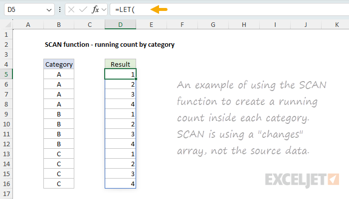
The SCAN function can also be used to create a running count by category. In the worksheet below, we have a list of categories (“A”, “B”, “C”) in the range B5:B16, and the goal is to create a running count for each category. The formula in D5 looks like this:
=LET(
    groups,B5:B16,
    changes,IF(groups<>VSTACK("",DROP(groups, -1)),1,0),
    SCAN(0,changes,LAMBDA(a,v,IF(v=1,1,a+1)))
)
This is a case where we need to create an intermediate array of changes before we can use the scan function. First, we define the variable groups to equal the range B5:B16. Then we set the variable changes to equal the result of this calculation:
IF(groups<>VSTACK("", DROP(groups, -1)), 1, 0)
The formula above uses VSTACK to add an empty string ("") at the beginning of the array, and DROP to remove the last value from the original array. This creates an array that is offset by one position, which allows us to compare each value with the previous value. For example, if the original array is {A,A,A,B,B,C,C}, after using VSTACK and DROP, we get:
| Original | Offset | Different? |
|---|---|---|
| A | "" | 1 |
| A | A | 0 |
| A | A | 0 |
| B | A | 1 |
| B | B | 0 |
| C | B | 1 |
| C | C | 0 |
The IF function then compares these arrays and returns 1 when values are different (indicating a category change) and 0 when they are the same (indicating we’re still in the same category). The result is the array below, which is assigned to the variable changes :
{1;0;0;0;1;0;0;0;1;0;0;0}
Finally, SCAN processes this array of changes. When it encounters a 1 (indicating a category change), it resets the counter to 1. When it encounters a 0 (indicating we’re still in the same category), it increments the previous count by 1. The result is a running count within each category.
SCAN with text values
SCAN can also be used to concatenate text values. To work with text values, set the initial_value to an empty string (""). The formula below creates a running concatenation of an array:
=SCAN("",{"a","b","c"},LAMBDA(a,v,a&v)) // returns {"a","ab","abc"}
You can see an example of this approach in the worksheet below, where we have text in column B and the formula in column D is
=SCAN("",B5:B16,LAMBDA(a,v,a&v))
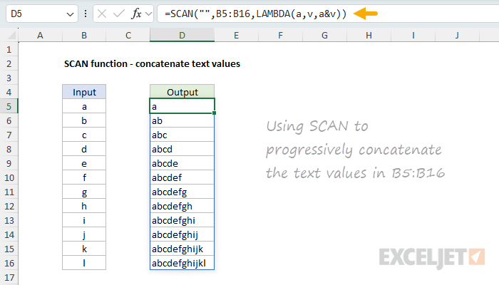
The result is a running concatenation of the text values in column B as seen in the worksheet above.
Note: let me know if you run into a good use case for SCAN with text values.
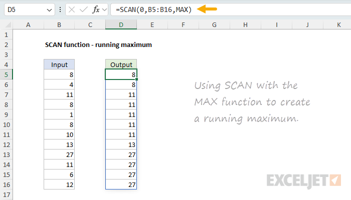
SCAN for a running MAX
The SCAN function can also be used to create a running MAX. In the worksheet below, we have a list of values in the range B5:B16 and the goal is to create a running maximum. The formula in D5 looks like this:
=SCAN(0,B5:B16,MAX)
The result is a list of running maximum values. Notice that the max value only changes when SCAN encounters a new maximum value.
Also, notice that this is a case where the abbreviated syntax for functions inside of SCAN works well, since MAX(a,v) works as needed. The equivalent “long form” formula would look like this:
=SCAN(0,B5:B16,LAMBDA(a,v,MAX(a,v)))
To create a running minimum, just replace the MAX function with the MIN function.
Note: In this example, we have set initial_value to zero because the values in column B will always be positive. If values could be negative, we need to supply an initial value that is less than or equal to the minimum value in the range. A general form for a running MAX that will work for any input values is: =SCAN(MIN(range),range,MAX) Excel power users will also sometimes use =SCAN(-9.99E+307,range,MAX) , since -9.99E+307 is the smallest number Excel can represent.
SCAN to find the longest winning streak
One interesting use of SCAN is to find the longest winning streak. This is traditionally a tricky problem to solve in Excel, but with SCAN, it’s fairly straightforward. In the worksheet below, we have a list of dates in column B, and column C contains a “W” or “L” to indicate a win or loss. The goal is to find the longest winning streak, which is 5 consecutive wins in this case. The formula in cell E5 looks like this:
=MAX(SCAN(0,C5:C16,LAMBDA(a,v,IF(v="w",a+1,0))))
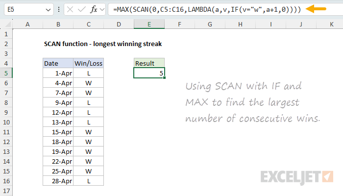
Notice the SCAN function is wrapped in the MAX function. Inside SCAN, we use the IF function to increment the accumulator by 1 if the value is “W”. Otherwise, we set the accumulator to 0. The result is a running count of consecutive wins. For the data shown above, the result from SCAN is an array like this:
{0;1;2;0;0;0;1;2;3;4;5;0}
This array is then passed to the MAX function, which returns the largest value in the array:
=MAX({0;1;2;0;0;0;1;2;3;4;5;0}) // returns 5
The final result is 5. Without the SCAN function, finding the longest winning streak is a lot more complicated. For a full explanation, see this article .
SCAN for compounded interest
The SCAN function can also be used to calculate compounded interest. In the worksheet below, we have variable inputs for starting balance, annual interest rate, and the number of years. The formula in E5 generates a sequence of years with the SEQUENCE function like this:
=SEQUENCE(C7) // returns {1;2;3;4;5;6;7;8;9;10}
The formula in F5 uses the SCAN function to calculate compound interest like this:
=SCAN(C5,E5#,LAMBDA(a,v,a*(1+C6)))
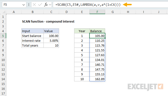
The initial_value is the starting balance in cell C5, the array is the sequence of years, and the calculation is the formula for compound interest. The final result is a list of ending balances for each year. Notice we use the spill range operator (E5#) to provide an array of years to the SCAN function. This allows the results to expand or contract based on the number of years provided. If we change the number of years in C7 to 15, SEQUENCE will output a list of all 15 years, and the SCAN function will generate a balance for the 5 additional years.
You can find another more advanced example of the SCAN function here: Modeling the 4% Retirement Rule in Excel .
Purpose
Return value
Syntax
=SEQUENCE(rows,[columns],[start],[step])
- rows - Number of rows to return.
- columns - [optional] Number of columns to return.
- start - [optional] Starting value (defaults to 1).
- step - [optional] Increment between each value (defaults to 1).
Using the SEQUENCE function
The SEQUENCE function generates a list of sequential numbers in an array. The array can be one-dimensional, or two-dimensional, controlled by rows and columns arguments. SEQUENCE can be used on its own to create an array of sequential numbers that spill directly on the worksheet. It can also be used to generate a numeric array inside another formula , a requirement that comes up frequently in more advanced formulas.
The SEQUENCE function takes four arguments : rows , columns , start , and step . All values default to 1. The rows and columns arguments control the number of rows and columns that should be generated in the output. For example, the formulas below generate numbers between 1 and 5 in rows and columns:
=SEQUENCE(5,1) // returns {1;2;3;4;5} in 5 rows
=SEQUENCE(1,5) // returns {1,2,3,4,5} in 5 columns
Note that the output from SEQUENCE is an array of values that will spill into adjacent cells. The formula below will create a 5 x 5 array that contains 25 cells with the values 1-25:
=SEQUENCE(5,5) // numbers 1-25 in a 5 x 5 array
The syntax for SEQUENCE indicates that rows is required and columns is optional. However, either can be omitted:
=SEQUENCE(5) // returns {1;2;3;4;5} in 5 rows
=SEQUENCE(,5) // returns {1,2,3,4,5} in 5 columns
The start argument is the starting point in the numeric sequence, and step controls the increment between each value. Both formulas below use a start value of 10 and a step value of 5:
=SEQUENCE(3,1,10,5) // returns {10;15;20} in 3 rows
=SEQUENCE(1,3,10,5) // returns {10,15,20} in 3 columns
Video: T he SEQUENCE function
Examples
In the example in the screen above, the formula in B4 is:
=SEQUENCE(10,5,0,3)
With this configuration, SEQUENCE returns an array of sequential numbers, 10 rows by 5 columns, starting at zero and incremented by 3. The result is 50 numbers starting at 0 and ending at 147, as shown in the screen.
Positive and negative
SEQUENCE can work with both positive and negative values. To count from -10 to zero in increments of 2 in rows, set rows to 6, columns to 1, start to -10, and step to 2:
=SEQUENCE(6,1,-10,2) // returns {-10;-8;-6;-4;-2;0}
To count down between 10 and zero:
=SEQUENCE(11,1,10,-1) // returns {10;9;8;7;6;5;4;3;2;1;0}
Sequence of dates
Because Excel dates are serial numbers , you can easily use SEQUENCE to generate sequential dates. For example, to generate a list of 10 days starting today in columns, you can use SEQUENCE with the TODAY function .
=SEQUENCE(1,10,TODAY(),1)
More details here . To generate a list of 12 dates corresponding to the first day of the month for all months in a year (2022 in this case) you can use SEQUENCE with the DATE and EDATE functions:
=EDATE(DATE(2022,1,1),SEQUENCE(12,1,0))
To generate a list of twelve-month names (instead of dates) you can wrap the formulas above in the TEXT function like this:
=TEXT(EDATE(DATE(2022,1,1),SEQUENCE(12,1,0)),"mmmm")
More information about these formulas here .
SEQUENCE with text
SEQUENCE generates numeric arrays. However, it is possible to use SEQUENCE to create arrays that contain text. For example, the formula below will generate a 5 x 5 array filled with “x”:
=REPT("x",SEQUENCE(5,5,1,0)) // 5 x 5 array of x's
SEQUENCE is configured ot return a 5 x 5 array of 1’s, which are fed into the REPT function with “x” as the text to repeat. By replacing “x” with an empty string, we can generate an empty 5 x 5 array:
=REPT("",SEQUENCE(5,5,1,0)) // empty 5 x 5 array
The formula below will generate an array that contains the 26 letters from A-Z:
=CHAR(SEQUENCE(26,,65)) // generate A-Z
The SEQUENCE function returns 26 numbers starting with 65. The CHAR function returns a specific character based on its ASCII number . The letter “A” is 65, and “Z” is 90, so the result is all 26 uppercase letters.
You can also use the MAKEARRAY function to generate an array that contains the result of a custom calculation.
