Purpose
Return value
Syntax
=SEARCH(find_text,within_text,[start_num])
- find_text - The substring to find.
- within_text - The text to search within.
- start_num - [optional] Starting position. Optional, defaults to 1.
Using the SEARCH function
The SEARCH function returns the position (as a number) of one text string inside another. In the most basic case, you can use SEARCH to locate the position of a substring in a text string. You can also use SEARCH to check if a cell contains specific text. SEARCH is not case-sensitive , which means it does not distinguish between uppercase and lowercase letters. In addition, SEARCH supports the use of wildcards like *?~, allowing more flexible search patterns. Here are a few key points to remember about the SEARCH function:
- SEARCH returns the position of one text string inside another as a number .
- When SEARCH cannot locate the search string, it returns a #VALUE error.
- If the search string appears more than once, SEARCH returns the first position .
- SEARCH is not case-sensitive and will treat “Apple” and “apple” as the same text strings.
- SEARCH does support wildcards like *?~ when searching for text.
- SEARCH will return 1 if the search string ( find_text ) is empty, which can cause a false positive when find_text is an empty cell.
Note: The SEARCH function is similar to the FIND function. Both functions return the position of one text string inside another. However, unlike FIND, SEARCH is not case-sensitive and does support wildcards.
Basic syntax
The basic syntax of the SEARCH function looks like this
SEARCH(find_text,within_text,[start_num])
- find_text : The text you want to find (the search string). This is a substring that Excel searches for within another text string. The text must be entered in double quotes if you are hardcoding the value into the formula. Otherwise, you can refer to a cell that contains the text.
- within_text : The text string that contains the text you want to find. Often, this is a cell reference that contains the text, but you can also hardcode a text string in double quotes.
- start_num (optional): The character at which to begin searching as a numeric position. The first character in within_text is considered position 1. If omitted, the search starts at the beginning of the within_text .
Basic example
The SEARCH function is designed to look inside a text string for a specific substring. When SEARCH locates the substring, it returns the position of the substring in the text as a number. If the substring is not found, SEARCH returns a #VALUE error. For example:
=SEARCH("p","apple") // returns 2
=SEARCH("z","apple") // returns #VALUE!
=SEARCH("apple","Pineapple") // returns 5
Note that text values entered directly into SEARCH must be enclosed in double quotes (""). Unlike the FIND function, the SEARCH function is not case-sensitive:
=SEARCH("a","Apple") // returns 1
=SEARCH("A","Apple") // returns 1
=SEARCH("Apple","Pineapple") // returns 5
The worksheet below shows the same examples translated into formulas based on cell references:
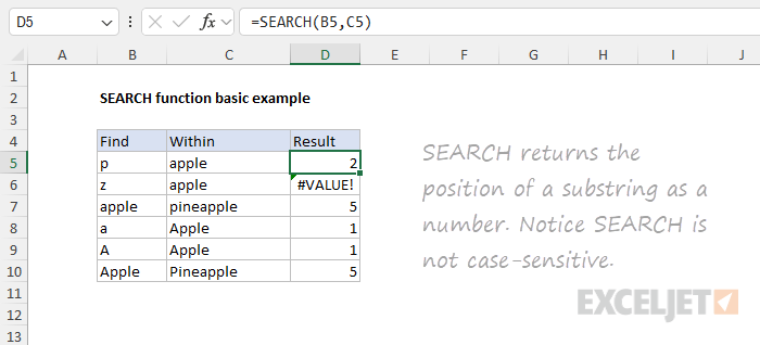
Again, notice that SEARCH is not case-sensitive, as seen in D8 and D10.
Forcing a TRUE or FALSE result
By default, the SEARCH function returns a number when a search string is found and a #VALUE! error when not. This is inconvenient in cases where you simply want to know if the search string has been found or not. To force a TRUE or FALSE result, you can nest the SEARCH function inside the ISNUMBER function . ISNUMBER returns TRUE for numeric values and FALSE for anything else. If SEARCH locates the substring, it returns the position as a number, and ISNUMBER returns TRUE:
=ISNUMBER(SEARCH("p","apple")) // returns TRUE
=ISNUMBER(SEARCH("z","apple")) // returns FALSE
If SEARCH doesn’t locate the substring, it returns an error, and ISNUMBER returns FALSE. This approach allows for support for wildcards in the search. For a more detailed explanation of this approach, with many more examples, see this example .
If cell contains
Once you have a TRUE or FALSE result, you can combine the SEARCH function with the IF function to create “if cell contains” logic. The generic pattern for this formula looks like this:
=IF(ISNUMBER(SEARCH(substring,A1)), "Yes", "No")
Instead of returning TRUE or FALSE, the formula above will return “Yes” if the substring is found and “No” if not. You can use the same idea to mark or “flag” items of interest. For example, in the worksheet below, we are using SEARCH with IF to flag email addresses that contain “abc” with an “x”.
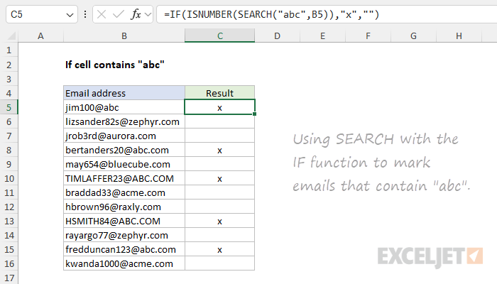
The formula in C5, copied down, is:
=IF(ISNUMBER(SEARCH("abc",B5)),"x","")
Start number
The SEARCH function has an optional argument called start_num that controls where SEARCH should begin looking for a substring. To find the first match of “x” in upper or lowercase, you can omit start_num , which defaults to 1:
=SEARCH("x","20 x 30 x 50") // returns 4
SEARCH returns 4 since the first “x” appears at position 4. To find the second “x”, enter 5 for start_num :
=SEARCH("x","20 x 30 x 50",5) // returns 9
In this case, SEARCH returns 9 since it starts searching after the first “x”. You can effectively find the second “x” in cell A1 in a single formula by using the SEARCH function twice like this:
=SEARCH("x",A1,SEARCH("x",A1)+1)
The inner SEARCH returns the location of the first “x”. We then add 1, and the result is used as the start_num in the outer SEARCH. The result is the location of the second “x” in cell A1.
Wildcards
Although SEARCH is not case-sensitive, it does support wildcards (*?~), which makes it a versatile tool for finding substrings in text. This allows for more complex searches, including basic pattern matching. For example, the question mark (?) wildcard matches any one character. The formula below looks for a 3-character substring beginning with “x” and ending in “y”:
=ISNUMBER(SEARCH("x?z","xyz")) // TRUE
=ISNUMBER(SEARCH("x?z","xbz")) // TRUE
=ISNUMBER(SEARCH("x?z","xyy")) // FALSE
The asterisk (*) wildcard is not as useful in the SEARCH function because SEARCH already looks for a substring . For example, it might seem like the following formula will test for a value that ends with “z”:
=SEARCH("*z",text)
However, because SEARCH automatically looks for a substring , the following formulas all return 1 as a result, even though the text in the first formula is the only text that ends with “z”:
=SEARCH("*z","XYZ") // returns 1
=SEARCH("*z","XYZXY") // returns 1
=SEARCH("*z","XYZXY123") // returns 1
=SEARCH("x*z","XYZXY123") // returns 1
However, it is possible to use the asterisk (*) wildcard like this:
=SEARCH("x*2*b","AAAXYZ123ABCZZZ") // returns 4
=SEARCH("x*2*b","NXYZ12563JKLB") // returns 2
Here we are looking for “x”, “2”, and “b” in that order, with any number of characters in between. Finally, use the tilde (~) as an escape character to indicate that the next character is a literal like this:
=SEARCH("~*","apple*") // returns 6
=SEARCH("~?","apple?") // returns 6
=SEARCH("~~","apple~") // returns 6
The above formulas use SEARCH to find a literal asterisk (*), question mark (?), and tilde (~) in that order.
More advanced formulas
The SEARCH function shows up in many more advanced formulas that work with text. SEARCH is often used instead of FIND when wildcards are needed or when the goal is to perform a case-insensitive search. Here are a few examples:
- Cell contains one of many things - tests a cell for more than one text string simultaneously, using wildcards for flexible matching.
- Sum if cells contain either x or y - sums numbers when associated cells contain one value or another, utilizing wildcard searches.
- Filter if text contains - extract values from a data set with “contains-type” logic, leveraging wildcards for comprehensive searching.
- Categorize text with keywords - return an appropriate category based on if a cell contains one of several text values, using wildcards to match patterns.
- Filter based on partial match - extract records from an Excel Table based on a partial match, using wildcards for pattern recognition.
Notes
- The SEARCH function returns the location of the first find_text in within_text as a number.
- SEARCH returns #VALUE if find_text is not found.
- Start_num is optional and defaults to 1.
- SEARCH returns 1 when find_text is empty. This can cause a false positive when find_text is an empty cell.
- SEARCH is not case-sensitive but does support wildcards.
- Use the FIND function for a case-sensitive search.
- SEARCH allows the wildcard characters question mark (?) and asterisk (), in find_text . ? matches any single character * matches any sequence of characters. To find a literal ? or * or ~, use a tilde (~) before the character, i.e. ~, ~?,~~.
Purpose
Return value
Syntax
=SUBSTITUTE(text,old_text,new_text,[instance_num])
- text - The text to change.
- old_text - The text to replace.
- new_text - The text to replace with.
- instance_num - [optional] The instance to replace. If not supplied, all instances are replaced.
Using the SUBSTITUTE function
The SUBSTITUTE function is a way to perform a find‑and‑replace with a formula. Use it when you know what text you want to change, but you don’t know (or care) where it appears in a text string. By default, SUBSTITUTE will replace all instances of a text string with another text string. Optionally, you can specify which instance of text to replace by providing a number. To completely remove matched text ( old_text ), enter an empty string ("") for the new_text argument.
Key features
- Replaces text by matching , not by position .
- Will replace all instances of matched text by default.
- Use instance_num to target only the 1st, 2nd, 3rd… match.
- Is case-sensitive and does not support wildcards.
- Works in all versions of Excel.
Because SUBSTITUTE doesn’t support wildcards, it can’t perform pattern matching. If you need pattern matching, see the REGEXREPLACE function , which brings the power of regular expressions to Excel formulas. If you want to replace text at a specific known position , see the REPLACE function .
- Example #1 – Basic usage
- Example #2 – Replace all
- Example #3 – Replace nth instance
- Example #4 – Replace line breaks
- Example #5 – Remove unwanted text
- Example #6 – Remove parentheses
- Related functions
- Notes
Example #1 - Basic usage
The SUBSTITUTE function is used to replace one text string with another using a generic syntax like this:
=SUBSTITUTE(text,old_text,new_text,[instance_num])
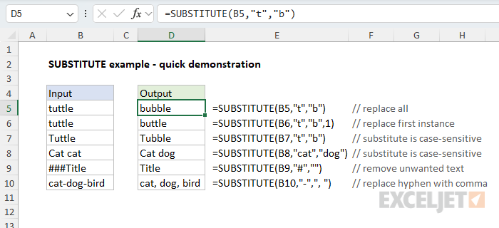
Where text is the value to process (typically a cell reference), old_text is the text to find, new_text is the text to replace with, and instance_num is an optional argument to target only a specific instance of old_text by number. You can see how this works below. The formulas starting in cell D5 look like this:
=SUBSTITUTE(B5,"t","b") // replace all t's with b's
=SUBSTITUTE(B6,"t","b",1) // replace first t with b
=SUBSTITUTE(B7,"t","b") // replace all t's with b's
=SUBSTITUTE(B8,"cat","dog") // replace cat with dog
=SUBSTITUTE(B9,"#","") // replace # with nothing
=SUBSTITUTE(B10,"-",", ") // replace hyphens with commas
Example #2 - Replace all
By default, the SUBSTITUTE function will replace all instances of one text string with another. You can see this behavior in the worksheet below, where we use SUBSTITUTE to replace periods (.) with hyphens (-). The formula in cell D5 looks like this:
=SUBSTITUTE(B5,".","-")
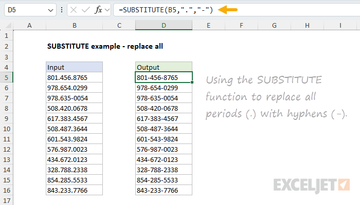
Notice the hyphen that already exists in cell B7 is unaffected.
Example #3 - Replace nth instance
By default, SUBSTITUTE will replace all instances of one text string with another. The optional fourth argument, called instance_num, can be used to replace just a specific instance. You can see this in the worksheet below, where we have configured SUBSTITUTE to replace only the second space with a hyphen. The formula in cell D5 copied down is:
=SUBSTITUTE(B5," ","-",2)
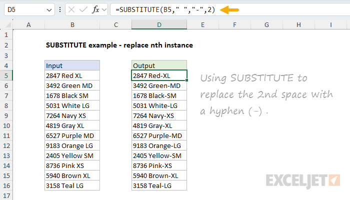
Notice that instance_num is provided as 2 to target the second space character.
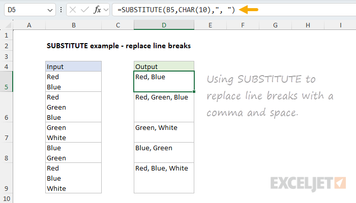
Example #4 - Replace line breaks
SUBSTITUTE can be combined with other functions to solve more difficult problems. The example below uses the SUBSTITUTE function to replace line breaks with a comma and a space. This is a tricky problem because the line breaks aren’t visible. However, because line breaks in Excel are ASCII character 10, we can use the CHAR function to inject a line break character for old_text inside SUBSTITUTE. The formula in cell D5 is:
=SUBSTITUTE(B5,CHAR(10),", ")
Example #5 - Remove unwanted text
You can use the SUBSTITUTE function to completely remove unwanted text by providing an empty string for the new_text argument. You can see this approach below, where we use SUBSTITUTE to strip all asterisks (*) from the numbers in column B. The formula in cell D5 looks like this:
=SUBSTITUTE(B5:B16,"*","")+0

Why add zero? Adding zero to the result forces Excel to convert text values to numbers when possible. You can see that it works in this case because the numbers in column D are now right-aligned. Also, notice we have provided the range B5:B16 as the text argument. Because we provide 12 values, SUBSTITUTE returns 12 results that spill into the range D5:D16.
Example #6 - Remove parentheses
SUBSTITUTE cannot replace more than one text string at a time. However, as a workaround, you can nest one SUBSTITUTE function inside another. You can see an example of this approach in the worksheet below, where we use SUBSTITUTE twice in one formula to remove the parentheses from the values in column B. This requires that we perform two replacements: one for the left parentheses and one for the right parentheses. The formula in D5 looks like this:
=SUBSTITUTE(SUBSTITUTE(B5,"(",""),")","")
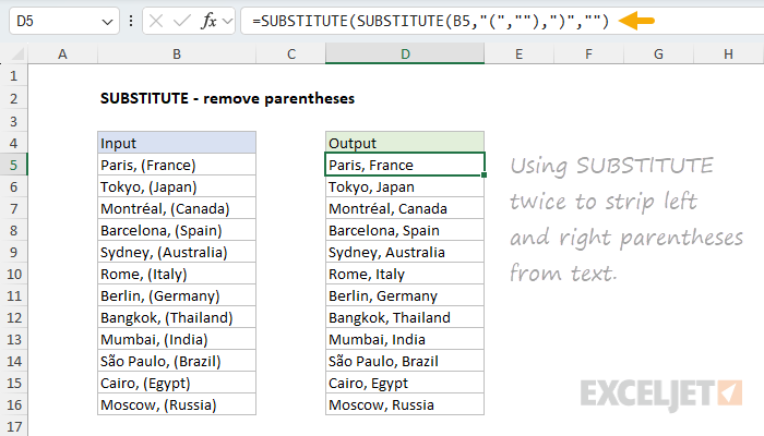
This is an example of nesting one SUBSTITUTE inside another. The inner SUBSTITUTE runs first, replacing the left parenthesis with an empty string. The result is returned directly to the outer SUBSTITUTE, which replaces the right parentheses with an empty string. The final result in column D contains no parentheses.
See a more advanced example of this approach in a formula to normalize telephone numbers .
Related functions
Excel contains several functions that can help you find and replace text:
- REPLACE – Replace text by position when you know the starting point.
- FIND / SEARCH – Find the numeric position of text.
- REGEXREPLACE – Pattern‑based find and replace (Excel 365 only).
Notes
- SUBSTITUTE replaces old_text with new_text in a text string.
- By default, all instances of old_text are replaced with new_text .
- Instance_num limits replacement to a particular instance of old_text .
- SUBSTITUTE is case-sensitive and does not support wildcards .
- Use REGEXREPLACE (Excel 365) for more advanced replacement scenarios.
- SUBSTITUTE can only perform one replacement at a time.
