Explanation
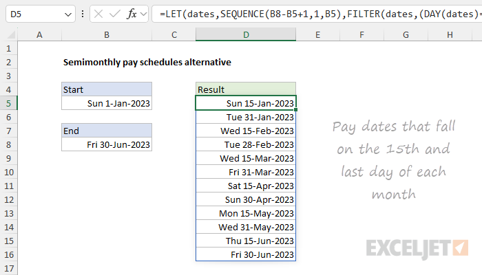
In this example, the goal is to create a list of pay dates that follow a semimonthly schedule. A semimonthly pay schedule means employees are paid twice a month, usually on fixed dates such as the 1st and 15th or the 15th and the last day of the month. This results in 24 pay periods over the course of a year. For example, in the worksheet shown above, payroll dates are the 1st and 15th of each month. In the worksheet shown above, the formula solves this problem in two steps. Step 1 is to generate a list of all dates between the start date and the end date. Step 2 is to filter those dates so that only those that land on the 1st and 15th remain. The formula in cell D5 looks like this:
=LET(dates,SEQUENCE(B8-B5+1,1,B5),FILTER(dates,(DAY(dates)=1)+(DAY(dates)=15)))
Background study
If you are not familiar with the SEQUENCE function, these links will help you get up to speed quickly:
- How to use the SEQUENCE function - overview
- The SEQUENCE function - 3 min video
- SEQUENCE of dates - 3 min video
- Dynamic Array Formulas - video training
Generating the dates
The first step is to generate all the dates, and this is done with the SEQUENCE function here:
SEQUENCE(B8-B5+1,1,B5) // generate all dates
The SEQUENCE function generates numeric sequences. Excel dates are just large serial numbers , so this part of the formula evaluates like this:
=SEQUENCE(B8-B5+1,1,B5)
=SEQUENCE(45107-44927+1,1,44927)
=SEQUENCE(181,1,44927)
Essentially, we are asking SEQUENCE for 181 sequential dates that start on 44927, which is the serial number for January 1, 2023, in Excel’s date system. The SEQUENCE generates an array that contains 181 dates, and these are defined as the variable “date” by the LET function :
=LET(dates,SEQUENCE(B8-B5+1,1,B5)
We use the LET function here to avoid redundancy. We need to use the full range of dates more than once in the formula, and creating this array once and assigning it to dates means the operation does not need to be repeated. This makes the formula easier to read and understand, and also improves performance.
Filtering the dates
At this point, we have a list of all dates within the target date range, and we have named the list dates . The next step is to filter the list to extract just the dates we are about: the paydays that occur on the 1st and 15th of each month. To do this, we use the FILTER function , which is configured like this:
FILTER(dates,(DAY(dates)=1)+(DAY(dates)=15))
The array in FILTER is given as dates , which contains all dates between January 1, 2023, and June 30, 2023. The include argument is set up like this:
(DAY(dates)=1)+(DAY(dates)=15) // 1st and 15th only
Here, we use the DAY function to extract just the day from the date, then use Boolean algebra with addition to construct an OR condition. In other words, we are filtering on dates that land on the 1st or the 15th day of each month. The final result from FILTER is an array of the 12 dates that land on the 1st and 15th of each month in the target date range. For more information on using addition (+) to create “OR logic”, see this short video: Array formulas with AND and OR logic .
Alternative formula - 15th and last
The formula above can be easily adapted to return payroll dates that follow different rules. For example, to return a list of payroll dates that fall on the 15th and last day of each month, you can use a formula like this:
=LET(dates,SEQUENCE(B8-B5+1,1,B5),FILTER(dates,(DAY(dates)=15)+(dates=EOMONTH(dates,0))))
The only difference in this formula is that the include logic inside FILTER has been adjusted like this:
(DAY(dates)=15)+(dates=EOMONTH(dates,0)) // 15th and last
The test for the 15th is the same. To test each for an “end of month” date, we use the EOMONTH function . Inside, EOMONTH, we provide 0 for months to return the last day of the month. As before, the two expressions are joined with addition (+) to create OR logic . The screen below shows the result:
WORKDAY adjustment
The formulas above work well, but they don’t check what day of the week pay dates land on. In the real world, companies often adjust pay dates that land on a holiday or weekend to the previous business day. So, for example, if the 15th of the month lands on a Saturday, the date is adjusted to Friday the 14th. To adjust dates that land on weekends or holidays back to the previous working day, you can use the WORKDAY function with a special configuration like this:
=WORKDAY(date+1,-1)
Essentially, we move forward one day, and then ask WORKDAY for the previous workday by providing -1 for days . In this configuration, WORKDAY returns the original date if it is a working day. Otherwise, WORKDAY steps back one day at a time and returns the first working day found. You can see the result in the worksheet below:

The original results from the “1st and 15h” formula appear in column D. Column F shows the adjusted dates. Notice that four dates have been shifted back to the previous working day.
All in one formula
It is possible to combine the formulas above into a single formula by piping the results from FILTER directly into the WORKDAY function like this:
=LET(dates,SEQUENCE(B8-B5+1,1,B5),WORKDAY(FILTER(dates,(DAY(dates)=1)+(DAY(dates)=15))+1,-1))
This formula will return the same results seen in column F, all in one step. In the same way, you can use the formula below to list adjusted dates for the 15th and last day of the month, like this:
=LET(dates,SEQUENCE(B8-B5+1,1,B5),WORKDAY(FILTER(dates,(DAY(dates)=15)+(dates=EOMONTH(dates,0)))+1,-1))
In both formulas, we’ve nested the FILTER formula inside the WORKDAY function as the start_date argument. This causes all the dates returned by FILTER to go through the WORKDAY, and only dates that land on non-working days are adjusted.
Note: To simplify things, I have not provided holidays to WORKDAY, but you can easily add this optional argument to make WORKDAY skip official holidays. See Previous working day for an example.
Legacy Excel
In older versions of Excel, there is no SEQUENCE function or FILTER function, so we can’t use the approach explained above. One option is to hardcode the first date into cell D5, then enter this formula in cell D6 and drag copy it down as needed:
=IF(DAY(D5)=1,D5+14,EOMONTH(D5,0)+1)
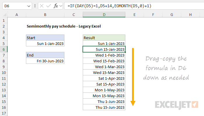
This formula uses the IF function and the DAY function to check the date in the “cell above” to see if it is the first of the month. If it is, IF returns the date + 14 days. If it is not the first of the month, we use the EOMONTH function to move to the end of the month, then add one day to land on the first day of the next month.
Alternative
To list pay dates that fall on the 15th and last day of the month in older versions of Excel, you can use the same basic process and a formula like this:
=IF(DAY(D5)=15,EOMONTH(D5,0),D5+15)
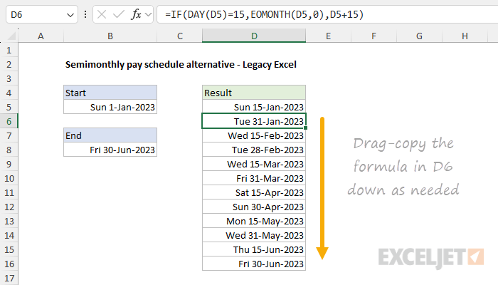
This formula assumes that the first date in D5 is either the 15th of a month or the last day of a month. As before, this formula uses the IF and DAY functions to check the date in the “cell above”. If the day is the 15th, we use the EOMONTH function to move to the end of the month. If the day is not the 15th, we assume it is the last day of the month and add 15 days.
Explanation
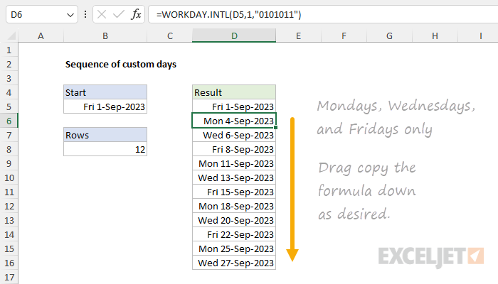
The goal is to generate a series of “custom” days of the week based on a start date entered in cell B5. For example, you might want to list sequential dates for any of the following combinations of days:
- Mondays, Wednesdays, and Fridays (as shown)
- Tuesdays, Thursdays, and Saturdays
- Tuesdays and Thursdays
- Mondays and Fridays
The number of dates to create (n) is entered in cell B8. If the start date or the number of dates to create is changed, the dates should be recalculated. In the current version of Excel, the easiest way to solve this problem is to use the SEQUENCE function inside the WORKDAY.INTL function. In older versions of Excel, you can also use the WORKDAY.INTL function and a more manual approach, as explained below.
WORKDAY.INTL function
The WORKDAY.INTL function takes a start date and returns the next workday based on a given offset value provided as the days argument. WORKDAY.INTL will automatically exclude Saturday and Sunday, and can optionally exclude dates that are holidays. The generic syntax for WORKDAY.INTL looks like this:
=WORKDAY.INTL(start_date,days,[weekend],[holidays])
- start_date - the date to start from
- days - the number of days to move forward or back
- weekend - a code to specify which days are weekends
- holidays - a list of dates that are non-working days
One of WORKDAY.INTL’s tricks is that it can be configured to treat any day of the week as a workday by providing the weekend argument as a 7-digit code that covers all seven days of the week, Monday through Saturday. In this scheme, a 1 indicates a weekend (non-working) day, and a 0 indicates a workday. The table below shows sample codes in column B and the workdays they define in column J:

This method is more flexible since it can define any day of the week as a weekend or workday. For example, to get the next workday that is a Monday, Wednesday, or Friday after a date in cell A1, you can use a formula like this:
=WORKDAY.INTL(A1,1,"0101011") // Mon, Wed, Fri
To get the next Tuesday or Thursday, you can use a formula like this:
=WORKDAY.INTL(A1,1,"1010111") // Tue, Thu
You can also use this feature to create a list of weekends only .
Note: weekend must be entered as a text string surrounded by double quotes ("") when using this feature.
Current Excel version
In the current version of Excel (Excel 2019+), the easiest way to solve this problem is to use the SEQUENCE function inside the WORKDAY.INTL function . In the workbook shown above, the formula in cell D5 is:
=WORKDAY.INTL(B5-1,SEQUENCE(B8),"0101011")
The inputs provided to WORKDAY.INTL are as follows:
- start_date - B5-1 (the day before the start date)
- days - array created by SEQUENCE (see below)
- weekend - “0101011” (code allowing Mon, Wed, and Fri only)
- holidays - omitted (could be supplied as a range of dates)
Working from the inside out, the SEQUENCE function is used to generate a sequential array of n numbers, where n comes from cell B8. With the number 12 in cell B8, SEQUENCE generates an array like this:
=SEQUENCE(B8)
=SEQUENCE(12)
={1;2;3;4;5;6;7;8;9;10;11;12}
Next, the start_date is calculated by subtracting 1 from the date in B5. We do this because we want to force WORKDAY.INTL to check the start date as well. If it is a Monday, Wednesday, or Friday, it should be included in the list:
=B5-1
=45170-1
=45169 // 31-Aug-2023
Excel dates are just large serial numbers , so the result is 45169, a number that represents 31-Aug-2023, the day before the start date in B5. Simplifying, we have:
=WORKDAY.INTL(45169,{1;2;3;4;5;6;7;8;9;10;11;12},"0101011")
Because days is given as an array with 12 numbers, WORKDAY.INTL returns 12 dates filtered by the code “0101011”, which treats only Mondays, Wednesdays, or Fridays as workdays. With this configuration, WORKDAY.INTL, returns the next 12 Saturdays and Sundays after 31-Aug-2023, skipping all Saturdays, Sundays, Tuesdays, and Thursdays. For more details on WORKDAY.INTL, see How to use the WORKDAY.INTL function .
Tuesdays and Thursdays
To create a list of Tuesdays and Thursdays, just update the weekend code like so:
=WORKDAY.INTL(B5-1,SEQUENCE(B8),"1010111") // Tue and Thu
List custom days between dates
To adapt this formula to list all Mondays, Wednesdays, and Fridays between two given dates ( start and end ), you can use the same basic idea in a formula like this:
=LET(dates,SEQUENCE(end-start+1,1,start),FILTER(dates,WORKDAY.INTL(dates-1,1,"0101011")=dates))
See this page for a detailed explanation of how this approach works.
Legacy Excel
In older versions of Excel, there is no SEQUENCE function, so we don’t have a simple way to request 12 dates at once. One simple solution is to set up the worksheet so that we can “drag copy” a formula that will return the next Saturday or Sunday after the “cell above”. First, enter this formula in cell D5:
=WORKDAY.INTL(B5-1,1,"0101011")
- start_date - B5-1 (day before the start date)
- days - 1 (i.e. next date)
- weekend - “1111100” (code allowing Mon, Wed, and Fri only)
To get the start_date , we subtract 1 day from the date in B5 to force WORKDAY.INTL to evaluate the start date in B5, like other dates. If the date in cell B5 is a Saturday or Sunday, it will be returned by the formula above. Otherwise, the next Saturday or Sunday will be returned. As explained above, the weekend argument is given as the code “1111100”, which tells WORKDAY.INTL to treat only Mondays, Wednesdays, and Fridays as workdays. Next, in cell D6, enter the formula below and copy the formula down as needed:
=WORKDAY.INTL(D5,1,"0101011")
As the formula is copied down, it begins with the date in the “cell above” and returns the next Monday, Wednesday, or Friday. Because the formula in cell D6 refers to the start date in cell B5, cell B5 still drives all results. The downside of this approach is that the formula in D5 is different from the formulas in cell D6 and below, so you must take care to keep them separate.
Conclusion
The WORKDAY.INTL function will calculate the next working day and can be customized with the “weekend” argument to treat any day of the week as a weekend or workday. The SEQUENCE function can be used within WORKDAY.INTL to create a dynamic list of custom days based on a start date and the number of dates you want. You can also combine WORKDAY.INTL with SEQUENCE and the FILTER function to list custom days between two given dates . In older versions of Excel without SEQUENCE, you can use a more manual approach to get the same results.
