Explanation
The goal is to generate a dynamic list of sequential working days with a formula. The start date should be a variable input, and weekends and holidays should be automatically excluded from the output. In the current version of Excel, the easiest way to solve this problem is to use the SEQUENCE function inside the WORKDAY.INTL function like this:
=WORKDAY.INTL(B5-1,SEQUENCE(12),1,B8:B11)
The result is a list of 12 working days, starting on September 1, 2023, and ending on September 19, 2023. Weekends and holidays are omitted from the result. Note that the number of dates to return is hardcoded into the formula as 12. However, this value could easily be exposed on the worksheet as another variable.
In older versions of Excel without the SEQUENCE function, you can use a more manual approach, which is also explained below.
SEQUENCE function
Working from the inside out, let’s look first at the SEQUENCE function . SEQUENCE is designed to generate numeric sequences in rows and/or columns. The generic syntax for SEQUENCE looks like this:
=SEQUENCE(rows,[columns],[start],[step])
In this example, the goal is to generate a sequence of 12 workdays that exclude weekends and holidays. The hard part of this problem is done by the WORKDAY.INTL function (see below), which is designed for this purpose. However, we need a way to ask WORKDAY.INTL to return 12 workdays, and this is where SEQUENCE comes into the picture. We use SEQUENCE inside WORKDAY.INTL to create a value for the days argument like this:
=SEQUENCE(12)
With the number 12 given for the rows argument, SEQUENCE returns an array that contains 12 numbers starting with 1 and ending with 12:
{1;2;3;4;5;6;7;8;9;10;11;12}
The other arguments not provided to SEQUENCE (columns, start, and step) all default to 1.
For more details, see How to use the SEQUENCE function .
WORKDAY.INTL function
The WORKDAY.INTL function takes a date and returns the next workday based on a given offset value provided as the days argument. WORKDAY.INTL will automatically exclude weekends and can optionally exclude dates that are holidays. The generic syntax for WORKDAY.INTL looks like this:
=WORKDAY.INTL(start_date,days,[weekend],[holidays])
The arguments inside WORKDAY.INTL have the following purpose:
- start_date - the date to start from
- days - the number of days to move forward or back
- weekend - the weekend scheme to use
- holidays - dates to be excluded as holidays
The screen below shows the basic operation of WORKDAY.INTL:
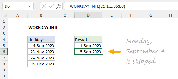
In the worksheet shown at the top, we use WORKDAY.INTL with the SEQUENCE function like this:
=WORKDAY.INTL(B5-1,SEQUENCE(12),1,B8:B11)
The inputs provided to WORKDAY.INTL are as follows:
- start_date - B5-1 (the day before the start date)
- days - array created by SEQUENCE
- weekend - 1 (Saturdays and Sundays)
- holidays - B8:B11 (dates that are holidays)
With the configuration above, WORKDAY.INTL starts on the day before the start date and calculates 12 workdays using the numbers returned by SEQUENCE as the days argument. After SEQUENCE runs, the formula looks like this:
=WORKDAY.INTL(B5-1,{1;2;3;4;5;6;7;8;9;10;11;12},1,B8:B11)
You can see now that we are asking WORKDAY.INTL for twelve results: the workday 1 day after the start date, the workday 2 days after the start date, the workday 3 days after the start date, and so on. The reason we start one day before the start date is to force WORKDAY.INTL to evaluate the start date as a potential weekend or holiday so that it can be excluded if necessary.
Notes: (1) weekend is optional and will default to 1 to exclude Saturdays and Sundays. (2) Holidays is an optional argument and can be omitted. (3) For more details on WORKDAY.INTL, see How to use the WORKDAY.INTL function .
Legacy Excel
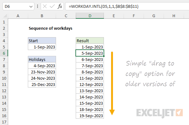
In older versions of Excel, there is no SEQUENCE function. This means we don’t have a simple way to calculate 12 workdays all at once. However, one simple solution is to use the WORKDAY.INTL and “drag copy” the formula down as needed. You can see this approach in the screen below. The formula in D6 looks like this:
=WORKDAY.INTL(D5,1,1,$B$8:$B$11)
The inputs to WORKDAY.INTL are as follows:
- start_date - D5 (the “cell above”)
- days - 1 (i.e. next workday)
- weekend - 1 (Saturdays and Sundays)
- holidays - $B$8:$B$11 (holidays as an absolute reference )
As the formula is copied down, it simply calculates the “next workday” after the date in the row above. If the date in D5 changes, all formulas will recalculate to return valid workdays.
Notes: (1) The formula in D5 is simply =B5 so that the start date in cell B5 is still functional. (2) One limitation of this formula is that it does not evaluate the start date as a potential non-working day.
More complete option
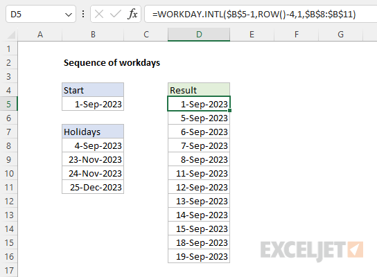
It is also possible to generate workdays with a more complex formula that uses the ROW function to determine the number of days to give WORKDAY.INTL. This allows the formula to evaluate the start date and makes it possible to copy the same formula into D5:D16. In the screen below, the formula in cell D5 is:
=WORKDAY.INTL($B$5-1,ROW()-4,1,$B$8:$B$11)
The inputs provided to WORKDAY.INTL are as follows:
- start_date - $B$5-1 (the day before the start date)
- days - ROW()-4 (we subtract 4 to start with 1)
- weekend - 1 (Saturdays and Sundays)
- holidays - $B$8:$B$11 (dates that are holidays)
We don’t have the SEQUENCE function to generate a value for days, but this approach mimics the same behavior. As before, we first subtract 1 day from the starting date in cell B5. We do this to force WORKDAY.INTL to evaluate the start date as a potential weekend or holiday. To create a value for days, we use the ROW function and subtract 4. We subtract 4 because the formula is entered in row 5, and we want to begin with 1. You will need to adjust this value if the formula is entered in a different row. As the formula is copied down, this value will increment.
For weekend , we provide 1, which is a code that configures WORKDAY.INTL to exclude Saturdays and Sundays. For holidays, we provide B8:B11, a range that contains dates that should be treated as non-working days. Notice that $B$5 and $B$8:$B$11 are entered as absolute references because we don’t want these values to change as the formula is copied. As the formula is copied down, the value returned by ROW() will increase, and each subsequent formula will display the next workday starting from the date in the cell above.
Explanation
The goal is to generate a series of dates one year apart. In the current version of Excel, the easiest way to do this is with the SEQUENCE function together with the DATE, YEAR, MONTH, and DAY functions. In older versions of Excel, you can use the same date functions and a more manual approach. Both methods are described below.
SEQUENCE function
The SEQUENCE function generates numeric arrays. For example, to generate the numbers 1 through 10 you can use SEQUENCE like this:
=SEQUENCE(10) // returns {1;2;3;4;5;6;7;8;9;10}
To solve this problem, we can use SEQUENCE to generate the years we need (2019-2030), then hand the years off to the DATE function along with the correct values for month and day. In the worksheet shown, the formula in D5 is:
=DATE(SEQUENCE(12,1,YEAR(B5)),MONTH(B5),DAY(B5))
Working from the inside out, the year, month, and day values from the date in B5 are first extracted with the YEAR, MONTH, and DAY functions. With the date May 1, 2019, in cell B5 YEAR returns 2019, MONTH returns 5, and DAY returns 1. The formula now looks like this:
=DATE(SEQUENCE(12,1,2019),5,1)
Next, the SEQUENCE function is evaluated with the following inputs:
- rows - 12
- columns - 1
- start - 2019
The result from SEQUENCE is an array with 12 years like this:
{2019;2020;2021;2022;2023;2024;2025;2026;2027;2028;2029;2030}
This array is returned as the year argument inside the DATE function:
=DATE({2019;2020;2021;2022;2023;2024;2025;2026;2027;2028;2029;2030},5,1)
Because we are giving the DATE function 12 values for the year, we are essentially asking for 12 separate dates, through a process known as " lifting “. The month is provided as 5 and day is provided as 1. The result is an array of 12 dates in serial number format like this:
{43586;43952;44317;44682;45047;45413;45778;46143;46508;46874;47239;47604}
These results spill into the range D5:D16. When these numbers are formatted as dates , the final result is a list of 12 dates, one year apart, beginning on May 1, 2019, and ending on May 1, 2030.
Year only option
It is also possible to use the same approach to create a list of years only, as seen in column F. The formula in cell F5 is:
=SEQUENCE(12,1,YEAR(B5))
SEQUENCE is configured to output 12 years as before. The value for start is provided by the YEAR function:
=YEAR(B5) // returns 2019
Since cell B5 contains the date May 1, 2019, the result is 2019. After YEAR is evaluated, we have:
=SEQUENCE(12,1,2019)
SEQUENCE then returns a list of 12 sequential years beginning in 2019 and incremented by 1:
{2019;2020;2021;2022;2023;2024;2025;2026;2027;2028;2029;2030}
The array lands in cell F5 and values spill into the range F5:F16.
Legacy Excel
To create a series of dates by year in an older version of Excel, we need to take a different approach, because there is no SEQUENCE function. One option is to use a formula like this:
=DATE(YEAR(date)+1,MONTH(date),DAY(date))
This formula first extracts the components of a date (year, month, day) with the DAY, MONTH, and YEAR functions. Then it adds 1 to the year value and returns the results to the DATE function which creates a new date. To adapt this formula to the worksheet shown, enter this formula in cell D5:
=B5
Note: This formula simply pulls in the start date from cell B5. The reason we do this is to maintain the workbook structure, with the start date in cell B5. Once we have the start date in cell D5, all formulas below can reference the “cell above”. An alternative would be to simply hardcode the start date into cell D5, but that would leave the start date in B5 “orphaned” with no purpose. It’s a good example of how the dynamic array created by SEQUENCE provides a more compact, elegant solution.
Next, in cell D6, enter the formula below:
=DATE(YEAR(D5)+1,MONTH(D5),DAY(D5))
To solve this formula, Excel first extracts the year, month, and day values from the date in D5, then adds 1 to the year value. Next, a new date is reassembled by the DATE function, using the same day and month, and year + 1 for the year:
=DATE(YEAR(D5)+1,MONTH(D5),DAY(D5))
=DATE(2019+1,5,1)
=DATE(2020,5,1)
="01-May-2020"
The result in D6 is the date May 1, 2020. As the formula is copied down, it returns a series of dates incremented by one year. The result should look like this:

If you only want a list of incremented years, enter this formula in cell D5:
=YEAR(B5)
Then in cell D6, enter and copy down this formula:
=D5+1
The result should look like this:

You can easily customize this formula if needed. For example, if you need a series of dates where every date is the first day of a new year, you can use a formula like this:
=DATE(YEAR(date)+1,1,1)
