Explanation
The goal is to generate a series of dates one year apart. In the current version of Excel, the easiest way to do this is with the SEQUENCE function together with the DATE, YEAR, MONTH, and DAY functions. In older versions of Excel, you can use the same date functions and a more manual approach. Both methods are described below.
SEQUENCE function
The SEQUENCE function generates numeric arrays. For example, to generate the numbers 1 through 10 you can use SEQUENCE like this:
=SEQUENCE(10) // returns {1;2;3;4;5;6;7;8;9;10}
To solve this problem, we can use SEQUENCE to generate the years we need (2019-2030), then hand the years off to the DATE function along with the correct values for month and day. In the worksheet shown, the formula in D5 is:
=DATE(SEQUENCE(12,1,YEAR(B5)),MONTH(B5),DAY(B5))
Working from the inside out, the year, month, and day values from the date in B5 are first extracted with the YEAR, MONTH, and DAY functions. With the date May 1, 2019, in cell B5 YEAR returns 2019, MONTH returns 5, and DAY returns 1. The formula now looks like this:
=DATE(SEQUENCE(12,1,2019),5,1)
Next, the SEQUENCE function is evaluated with the following inputs:
- rows - 12
- columns - 1
- start - 2019
The result from SEQUENCE is an array with 12 years like this:
{2019;2020;2021;2022;2023;2024;2025;2026;2027;2028;2029;2030}
This array is returned as the year argument inside the DATE function:
=DATE({2019;2020;2021;2022;2023;2024;2025;2026;2027;2028;2029;2030},5,1)
Because we are giving the DATE function 12 values for the year, we are essentially asking for 12 separate dates, through a process known as " lifting “. The month is provided as 5 and day is provided as 1. The result is an array of 12 dates in serial number format like this:
{43586;43952;44317;44682;45047;45413;45778;46143;46508;46874;47239;47604}
These results spill into the range D5:D16. When these numbers are formatted as dates , the final result is a list of 12 dates, one year apart, beginning on May 1, 2019, and ending on May 1, 2030.
Year only option
It is also possible to use the same approach to create a list of years only, as seen in column F. The formula in cell F5 is:
=SEQUENCE(12,1,YEAR(B5))
SEQUENCE is configured to output 12 years as before. The value for start is provided by the YEAR function:
=YEAR(B5) // returns 2019
Since cell B5 contains the date May 1, 2019, the result is 2019. After YEAR is evaluated, we have:
=SEQUENCE(12,1,2019)
SEQUENCE then returns a list of 12 sequential years beginning in 2019 and incremented by 1:
{2019;2020;2021;2022;2023;2024;2025;2026;2027;2028;2029;2030}
The array lands in cell F5 and values spill into the range F5:F16.
Legacy Excel
To create a series of dates by year in an older version of Excel, we need to take a different approach, because there is no SEQUENCE function. One option is to use a formula like this:
=DATE(YEAR(date)+1,MONTH(date),DAY(date))
This formula first extracts the components of a date (year, month, day) with the DAY, MONTH, and YEAR functions. Then it adds 1 to the year value and returns the results to the DATE function which creates a new date. To adapt this formula to the worksheet shown, enter this formula in cell D5:
=B5
Note: This formula simply pulls in the start date from cell B5. The reason we do this is to maintain the workbook structure, with the start date in cell B5. Once we have the start date in cell D5, all formulas below can reference the “cell above”. An alternative would be to simply hardcode the start date into cell D5, but that would leave the start date in B5 “orphaned” with no purpose. It’s a good example of how the dynamic array created by SEQUENCE provides a more compact, elegant solution.
Next, in cell D6, enter the formula below:
=DATE(YEAR(D5)+1,MONTH(D5),DAY(D5))
To solve this formula, Excel first extracts the year, month, and day values from the date in D5, then adds 1 to the year value. Next, a new date is reassembled by the DATE function, using the same day and month, and year + 1 for the year:
=DATE(YEAR(D5)+1,MONTH(D5),DAY(D5))
=DATE(2019+1,5,1)
=DATE(2020,5,1)
="01-May-2020"
The result in D6 is the date May 1, 2020. As the formula is copied down, it returns a series of dates incremented by one year. The result should look like this:

If you only want a list of incremented years, enter this formula in cell D5:
=YEAR(B5)
Then in cell D6, enter and copy down this formula:
=D5+1
The result should look like this:

You can easily customize this formula if needed. For example, if you need a series of dates where every date is the first day of a new year, you can use a formula like this:
=DATE(YEAR(date)+1,1,1)
Explanation
In this example, the goal is to list the 10 most frequently occurring text values in a range, in descending order by count, as seen in the range in E5:F14. This is an advanced formula that requires a number of nested functions. However, it is an excellent example of the power of dynamic array formulas in Excel . For convenience, data is the named range B5:B104. This range contains 100 random color names.
Get unique values
The first step in this problem is to get a list of unique colors from the data. This is easy to do with the UNIQUE function :
UNIQUE(data) // get unique colors
Since there 23 unique colors in B5:B104, UNIQUE returns an array containing 23 color names:
{"Violet";"Maroon";"Blue";"Pink";"Lime";"Navy";"Yellow";"White";"Cyan";"Teal";"Gold";"Orange";"Peach";"Black";"Turquoise";"Tan";"Red";"Green";"Gray";"Indigo";"Brown";"Purple";"Silver"}
Count unique values
Now that we have a list of values, the next step is to get a count for each unique value. This can be done with the COUNTIF function like this:
=COUNTIF(data,UNIQUE(data))
Here, the UNIQUE function returns the unique values in the data as the criteria argument, and COUNTIF calculates a count for each value. The result is an array with 23 counts like this:
{11;5;4;9;3;4;4;7;3;8;2;5;6;5;3;2;3;3;4;4;3;1;1}
We now have the basic ingredients we need to solve the problem.
Combine values and counts
The next step is to combine the list of unique colors with the counts to form the two-column table seen in column E and F. This can be done with the HSTACK function , which is designed to combine arrays horizontally. We can use HSTACK like this:
=HSTACK(UNIQUE(data),COUNTIF(data,UNIQUE(data)))
The result from HSTACK is a list of 23 unique colors on the left, combined with 23 counts on the right:
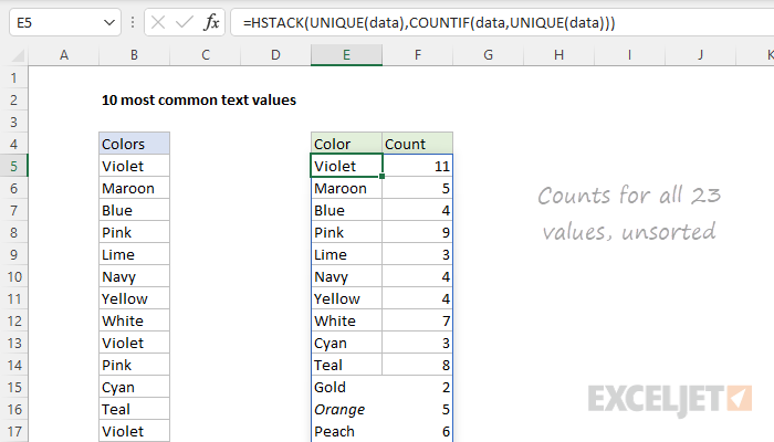
We are getting close to a solution, but we still need to reorder the list to show the highest counts first, and drop all but the top 10 counts.
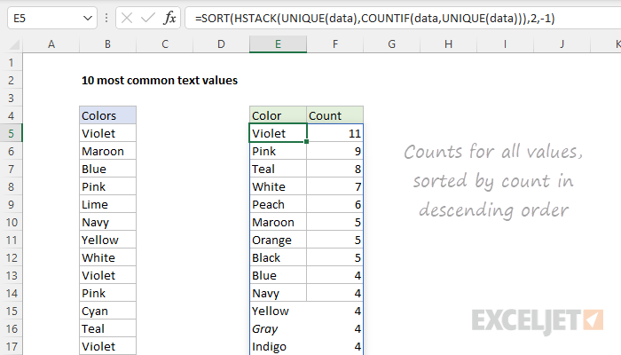
Sort by count
To sort the table by count, we can use the SORT function like this:
=SORT(HSTACK(UNIQUE(data),COUNTIF(data,UNIQUE(data))),2,-1)
Now we have the values sorted by count in descending order:
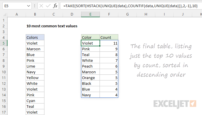
Top 10 values by count
The final step is to remove all but the top 10 values. The easiest way to do this is with the TAKE function , which is designed to extract rows and columns from arrays. In this case, we want the first 10 rows, so we provide 10 for rows:
=TAKE(SORT(HSTACK(UNIQUE(data),COUNTIF(data,UNIQUE(data))),2,-1),10)
The screen below shows the output of this formula:
Optimize
The formula above works fine, but it is a bit inefficient, since UNIQUE values are calculated twice. This might impact performance in larger sets of data. To streamline the formula, we can use the LET function . The LET function is used to declare and assign values to variables. In this case, we can use LET like this:
=LET(u,UNIQUE(data),TAKE(SORT(HSTACK(u,COUNTIF(data,u)),2,-1),10))
Here, we use UNIQUE to get unique values and assign the result to a variable named u . Then we replace UNIQUE(data) with u where it occurs in the formula. The result is that UNIQUE values are calculated just one time.
