Explanation
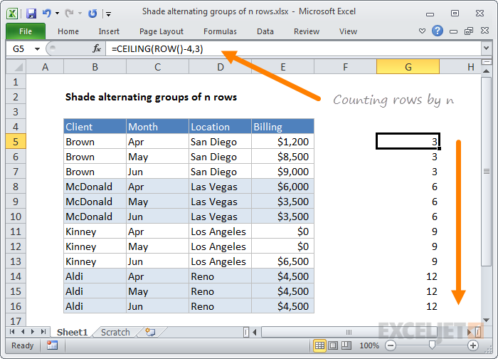
Working from the inside out, we first “normalize” row numbers to begin with 1 using the ROW function and an offset:
ROW()-offset
In this case, the first row of data is in row 5, so we use an offset of 4:
ROW()-4 // 1 in row 5
ROW()-4 // 2 in row 6
ROW()-4 // 3 in row 7
etc.
The result goes into the CEILING function, which rounds incoming values up to a given multiple of n. Essentially, the CEILING function counts by a given multiple of n:
This count is then divided by n to count by groups of n, starting with 1:

Finally, the ISEVEN function is used to force a TRUE result for all even row groups, which triggers the conditional formatting.
Odd row groups return FALSE so no conditional formatting is applied.
Shade first group
To shade rows starting with the first group of n rows, instead of the second, replace ISEVEN with ISODD:
=ISODD(CEILING(ROW()-offset,n)/n)
Explanation
Data validation rules are triggered when a user adds or changes a cell value.
The ISNUMBER function returns TRUE when a value is numeric and FALSE if not. As a result, all numeric input will pass validation.
Be aware that numeric input includes dates and times, whole numbers, and decimal values.
Note: Cell references in data validation formulas are relative to the upper left cell in the range selected when the validation rule is defined, in this case, C5.
Data Validation Guide | Data Validation Formulas | Dependent Dropdown Lists
