Substitute Function

Purpose

Return value

Syntax

=SUBSTITUTE(text,old_text,new_text,[instance_num])

• text - The text to change.
• old_text - The text to replace.
• new_text - The text to replace with.
• instance_num - [optional] The instance to replace. If not supplied, all instances are replaced.

Using the SUBSTITUTE function

The SUBSTITUTE function is a way to perform a find‑and‑replace with a formula. Use it when you know what text you want to change, but you don’t know (or care) where it appears in a text string. By default, SUBSTITUTE will replace all instances of a text string with another text string. Optionally, you can specify which instance of text to replace by providing a number. To completely remove matched text ( old_text ), enter an empty string ("") for the new_text argument.

Key features

• Replaces text by matching , not by position .
• Will replace all instances of matched text by default.
• Use instance_num to target only the 1st, 2nd, 3rd… match.
• Is case-sensitive and does not support wildcards.
• Works in all versions of Excel.

Because SUBSTITUTE doesn’t support wildcards, it can’t perform pattern matching. If you need pattern matching, see the REGEXREPLACE function , which brings the power of regular expressions to Excel formulas. If you want to replace text at a specific known position , see the REPLACE function .

• Example #1 – Basic usage
• Example #2 – Replace all
• Example #3 – Replace nth instance
• Example #4 – Replace line breaks
• Example #5 – Remove unwanted text
• Example #6 – Remove parentheses
• Related functions
• Notes

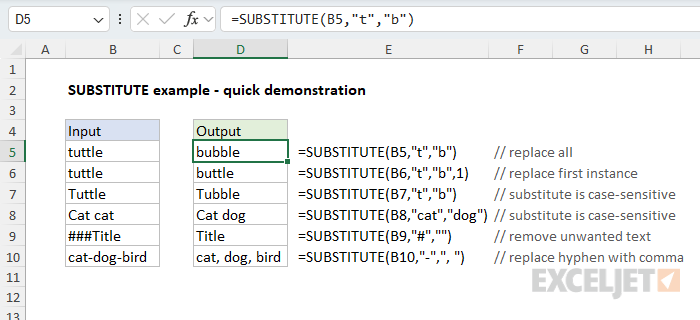
Example #1 - Basic usage

The SUBSTITUTE function is used to replace one text string with another using a generic syntax like this:

=SUBSTITUTE(text,old_text,new_text,[instance_num])

Where text is the value to process (typically a cell reference), old_text is the text to find, new_text is the text to replace with, and instance_num is an optional argument to target only a specific instance of old_text by number. You can see how this works below. The formulas starting in cell D5 look like this:

=SUBSTITUTE(B5,"t","b") // replace all t's with b's
=SUBSTITUTE(B6,"t","b",1) // replace first t with b
=SUBSTITUTE(B7,"t","b") // replace all t's with b's
=SUBSTITUTE(B8,"cat","dog") // replace cat with dog
=SUBSTITUTE(B9,"#","") // replace # with nothing
=SUBSTITUTE(B10,"-",", ") // replace hyphens with commas

Example #2 - Replace all

By default, the SUBSTITUTE function will replace all instances of one text string with another. You can see this behavior in the worksheet below, where we use SUBSTITUTE to replace periods (.) with hyphens (-). The formula in cell D5 looks like this:

=SUBSTITUTE(B5,".","-")

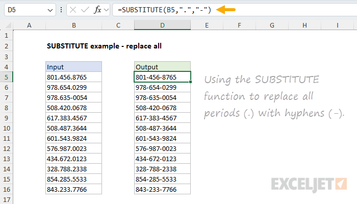
Notice the hyphen that already exists in cell B7 is unaffected.

Example #3 - Replace nth instance

By default, SUBSTITUTE will replace all instances of one text string with another. The optional fourth argument, called instance_num, can be used to replace just a specific instance. You can see this in the worksheet below, where we have configured SUBSTITUTE to replace only the second space with a hyphen. The formula in cell D5 copied down is:

=SUBSTITUTE(B5," ","-",2)

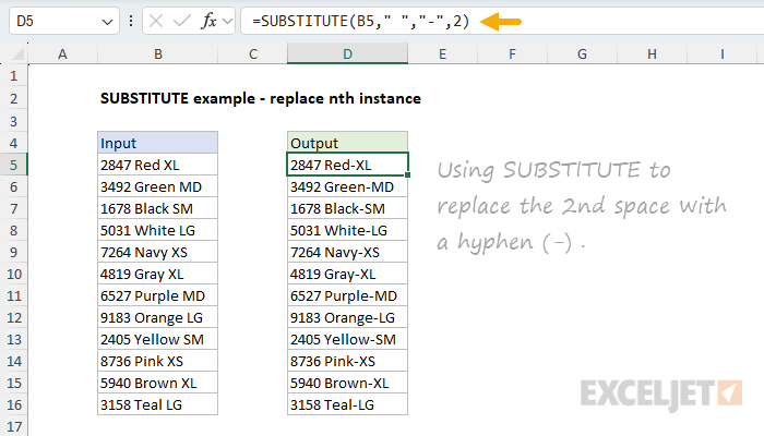
Notice that instance_num is provided as 2 to target the second space character.

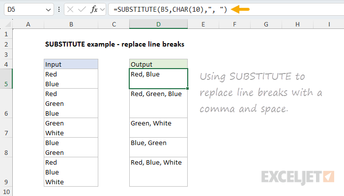
Example #4 - Replace line breaks

SUBSTITUTE can be combined with other functions to solve more difficult problems. The example below uses the SUBSTITUTE function to replace line breaks with a comma and a space. This is a tricky problem because the line breaks aren’t visible. However, because line breaks in Excel are ASCII character 10, we can use the CHAR function to inject a line break character for old_text inside SUBSTITUTE. The formula in cell D5 is:

=SUBSTITUTE(B5,CHAR(10),", ")

Example #5 - Remove unwanted text

You can use the SUBSTITUTE function to completely remove unwanted text by providing an empty string for the new_text argument. You can see this approach below, where we use SUBSTITUTE to strip all asterisks (*) from the numbers in column B. The formula in cell D5 looks like this:

=SUBSTITUTE(B5:B16,"*","")+0

Why add zero? Adding zero to the result forces Excel to convert text values to numbers when possible. You can see that it works in this case because the numbers in column D are now right-aligned. Also, notice we have provided the range B5:B16 as the text argument. Because we provide 12 values, SUBSTITUTE returns 12 results that spill into the range D5:D16.

Example #6 - Remove parentheses

SUBSTITUTE cannot replace more than one text string at a time. However, as a workaround, you can nest one SUBSTITUTE function inside another. You can see an example of this approach in the worksheet below, where we use SUBSTITUTE twice in one formula to remove the parentheses from the values in column B. This requires that we perform two replacements: one for the left parentheses and one for the right parentheses. The formula in D5 looks like this:

=SUBSTITUTE(SUBSTITUTE(B5,"(",""),")","")

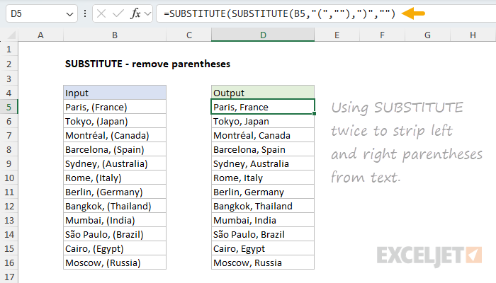
This is an example of nesting one SUBSTITUTE inside another. The inner SUBSTITUTE runs first, replacing the left parenthesis with an empty string. The result is returned directly to the outer SUBSTITUTE, which replaces the right parentheses with an empty string. The final result in column D contains no parentheses.

See a more advanced example of this approach in a formula to normalize telephone numbers .

Related functions

Excel contains several functions that can help you find and replace text:

• REPLACE – Replace text by position when you know the starting point.
• FIND / SEARCH – Find the numeric position of text.
• REGEXREPLACE – Pattern‑based find and replace (Excel 365 only).

Notes

• SUBSTITUTE replaces old_text with new_text in a text string.
• By default, all instances of old_text are replaced with new_text .
• Instance_num limits replacement to a particular instance of old_text .
• SUBSTITUTE is case-sensitive and does not support wildcards .
• Use REGEXREPLACE (Excel 365) for more advanced replacement scenarios.
• SUBSTITUTE can only perform one replacement at a time.

Purpose

Return value

Syntax

=TEXT(value,format_text)

• value - The number to convert.
• format_text - The number format to use.

Using the TEXT function

The TEXT function in Excel is a tool for formatting numbers, dates, and times as text. The purpose of the TEXT function is to convert a number to text using a specified format code. TEXT is most often used to control the formatting of a number embedded into a text string. However, TEXT is also a clever way to test dates in more advanced formulas (see below for an example).

• Syntax and example
• Why do we need the TEXT function?
• TEXT with dates
• TEXT with times
• TEXT with percentages
• Using TEXT in other formulas
• Notes

Syntax and example

The TEXT function takes two arguments, value and format_text .

• Value is the number to be formatted as text and should be a numeric value. Most often, this is a cell reference like A1. Note that the value must be a number for TEXT to do anything. If the value is already text, no formatting will be applied.
• Format_text is a text string that contains the format codes to apply to value . Note that format_text must be enclosed in double quotes (""), and must contain valid number format codes.

Assume cell A1 contains the number 1500.35, and your goal is to display the number as “$1,500.35”. You can do that by providing the number format “$#,##0.00” with TEXT like this:

=TEXT(A1,"$#,##0.00") // returns "$150.35"

The codes provided in format_codes can be adjusted to display decimal numbers, percentages, dates, times, and more.

Excel provides a huge number of codes that can be used to format numbers, including dates, times, currency, percentages, and more. For a detailed overview with many examples, see Excel Custom Number Formats .

Why do we need the TEXT function?

Why do we need the TEXT function? Can’t we just apply Excel’s built-in number formatting to format numbers in a worksheet? Yes. In general, you should always try to use regular number formatting first because it preserves the numeric value underneath. Keeping the number allows it to be used in standard numeric calculations.

The TEXT function, by contrast, actually converts a number to text. The result is text , so numbers returned by TEXT can’t be used in numeric calculations . However, there are still many situations where TEXT is quite helpful. The most common example is when you need to embed a number inside a text string. For example, assume we have the date 20-Oct-2024 in cell A1 and want to display a message like “The date is October 20, 2024”. If we simply concatenate the text to cell A1 like this:

="The date is "&A1 // returns "The date is 45585"

We end up with: “The date is 45585”. Why? This happens because the date formatting applied to cell A1 is not part of the number, which is 45585 in Excel’s date system . The formatting is not available during concatenation. To include a formatted date in a text string, we need to use the TEXT function to control formatting like this:

="The date is "&TEXT(A1,"mmmm d, yyyy")

This formula returns the date in a readable format like “The date is October 20, 2024”.

The TEXT function is especially useful when concatenating numbers and text. If you are new to the concept of concatenation, see How to concatenate in Excel .

TEXT with dates

With the date October 21, 2024, in cell A1, the TEXT function can be used like this:

=TEXT(A1,"dd-mmm-yy") // returns"24-Oct-2024"
=TEXT(A1,"mmmm d") // returns "October 21"

In the worksheet below, you can see how the TEXT function can be used to apply a variety of date formats to the date in cell B5:

The formulas used in column D are below. The result is shown after the “//” marker.

="The year is "&TEXT($B$5,"yyyy") // "The year is 2024"
="The month is "&TEXT($B$5,"mmmm") // "The month is October"
="The month is "&TEXT($B$5,"mmm") // "The month is Oct"
="The month is "&TEXT($B$5,"mm") // "The month is 10"
="The day is "&TEXT($B$5,"dddd") // "The day is Monday"
="The day is "&TEXT($B$5,"ddd") // "The day is Mon"
="The day is "&TEXT($B$5,"dd") // "The day is 21"
="The day is "&TEXT($B$5,"ddd, mmm d") // "The day is Mon, Oct 21"

TEXT with times

TEXT can format times as well as dates. For example, with the time 3:15 PM in cell A1, the TEXT function can print the time in a 24-hour format like this:

="The time is "&TEXT(A1,"hh:mm") // returns "The time is 15:00"

In the worksheet below, TEXT is configured to display the time in cell B5 in various ways:

The formulas used in column D are below. The result is shown after the “//” marker.

="The hour is "&TEXT($B$5,"h AM/PM") // "The hour is 3 PM"
="The hour is "&TEXT($B$5,"hh") // "The hour is 15"
="The minutes are "&RIGHT(TEXT($B$5,"hhmm"),2) // "The minutes are 15"
="The AM/PM is "&TEXT($B$5,"AM/PM") // "The AM/PM is PM"
="The time is "&TEXT($B$5,"hhmm") // "The time is 1515"
="The time is "&TEXT($B$5,"hh:mm") // "The time is 15:15"
="The time is "&TEXT($B$5,"h:mm AM/PM") // "The time is 3:15 PM"

Note that the formula in D7 is not like the others. Because the code “mm” conflicts with the date formatting codes for “month” when used alone, we use the format code “hhmm”. Then we use the RIGHT function to extract just the two characters to the right, which are minutes.

TEXT with percentages

With the number 0.537 in cell A1, TEXT can be used to apply percentage formatting like this:

=TEXT(A1,"0.0%") // returns "53.7%"
=TEXT(A1,"0%") // returns "54%"

In the worksheet below, we use the TEXT function together with the IFS function to report the gain or loss as a percentage in column F. The formula in F5, copied down, looks like this:

=IFS(D5>0,"Up "&TEXT(D5,"0.0%"),D5<0,"Down "&TEXT(D5,"0.0%"),D5=0,"Unchanged")

The IFS function is used to control the flow of the formula by testing for three conditions. If the change is greater than zero, IFS returns:

"Up "&TEXT(D5,"0.0%")

If the change is less than zero, IFS returns:

"Down "&TEXT(D5,"0.0%")

Finally, if the change equals zero, IFS returns the message “Unchanged”:

"Unchanged"

The result in column F is that each row has a custom message that depends on whether the change is positive, negative, or zero.

Using TEXT in other formulas

The TEXT function is surprisingly versatile and turns up in many other advanced formulas because it is so good an extracting useful information from a number. For example, in the worksheet below, the goal is to mark dates that occur in the same month and year with an “x”. The TEXT provides an elegant way to do this in a simple formula.

For a detailed explanation of how this formula works, see this page . Here is a related example of the TEXT function used to sort birthdays while ignoring the year, useful when you want to see a list of birthdays in the coming year.

Notes

• The TEXT function always returns text.
• Value must be a numeric value.
• Format_text must appear in double quotation marks.
• The TEXT function can be used with custom number formats
• TEXT always returns text . To keep the number, use standard number formatting .