Explanation
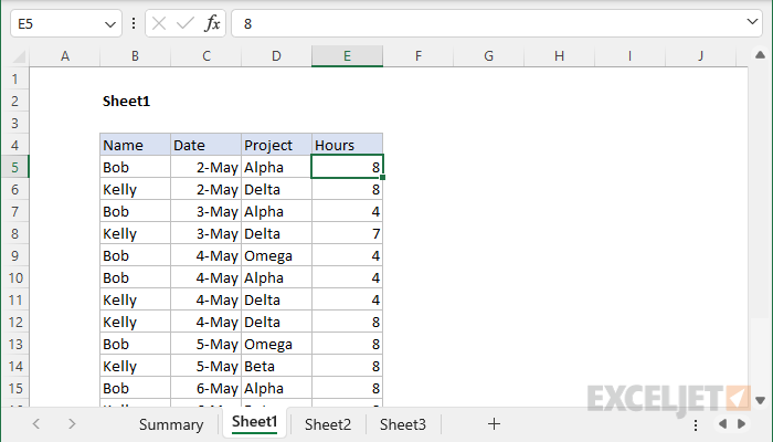
In this example, the goal is to sum hours per project across three different worksheets: Sheet1, Sheet2, and Sheet3. The data on each of the three sheets has the same structure as Sheet1, as seen below:
3D reference won’t work
Before we look at a solution, let’s look at something that doesn’t work. You might wonder if we can provide the SUMIF function with a 3D reference like this:
Sheet1:Sheet3!D5:D16
This is the standard 3D reference syntax, but if you try to use it with SUMIF, you’ll get a #VALUE error. The problem is that SUMIFS, COUNTIFS, AVERAGEIFS, etc. are in a group of functions that do not support 3D references.
Workaround with INDIRECT
To workaround this problem we can use a named range “sheets” that holds the name of each worksheet that should be included in the calculation. In the example shown, sheets is the named range B5:B7, which holds three values: “Sheet1”, “Sheet2”, and “Sheet3”. The formula in F5 is:
=SUMPRODUCT(SUMIF(INDIRECT("'"&sheets&"'!"&"D5:D16"),E5,INDIRECT("'"&sheets&"'!"&"E5:E16")))
Notice we are concatenating the sheet names to the ranges we need to work with. Once the concatenation is performed, the formula looks like this:
=SUMPRODUCT(SUMIF(INDIRECT({"'Sheet1'!D5:D16";"'Sheet2'!D5:D16";"'Sheet3'!D5:D16"}),E5,INDIRECT({"'Sheet1'!E5:E16";"'Sheet2'!E5:E16";"'Sheet3'!E5:E16"})))
Notice we now have complete references based on the three sheet names provided in sheets (B5:B7). However, because we assembled these references with concatenation, these values are not actual cell references but are in fact text values . To coerce these values into valid cell references we use the INDIRECT function .
INDIRECT converts the text values to valid references and returns the result to the SUMIF function for the range and sum_range arguments. The value for criteria is provided by the reference to cell E5 (“Alpha”), which changes as the formula is copied down the column. Because the named range “sheets” contains three values, SUMIF actually runs three times, one for each reference. The result is an array with three results like this:
{24;20;20}
This array is returned directly to the SUMPRODUCT function:
=SUMPRODUCT({24;20;20})
With a single array to process, SUMPRODUCT sums the array and returns 64 for the Alpha project in cell F5. This number is the total number of hours logged to the Alpha project in all three worksheets. As the formula is copied down, it returns a total for each project shown in column E.
Note: In the latest version of Excel, you can use the SUM function instead of the SUMPRODUCT function with the same result. In Legacy Excel , SUMPRODUCT is used frequently because it can handle arrays natively without requiring Ctrl-Shift-Enter.
Explanation
In this example, the goal is to create a formula that will sum values in a range that may contain errors. A common problem in Excel is that errors in data show up in the results of other formulas. For example, in the worksheet shown, the SUM function is used to sum the named range data (D5:D15) . Because the range D5:D15, the SUM function itself returns #N/A. The formula in cell F5 is:
=SUM(data) // returns #N/A
Ideally, the errors can be resolved by entering the missing data, and the SUM function will start working again. In fact, it is often helpful when summary calculations display errors, because it signals there are problems in the data that should be investigated. However, there are situations where you want to ignore errors and sum the available numbers. In this article, we look at three different formula options.
SUMIF
One option is to use the SUMIF function with the not equal to (<>) operator like this:
=SUMIF(data,"<>#N/A")
This is a relatively simple formula and it works fine as long as the range contains only #N/A errors. SUMIF returns the sum of values not equal to #N/A. However, if another type of error occurs, the SUMIF function will itself return an error. For example if the #DIV/0! error appears in the data, SUMIF will return #DIV/0!.
AGGREGATE
Another more robust option is to use the AGGREGATE function . In cell F7, AGGREGATE is configured to sum and ignore errors by setting function_num to 9, and options to 6:
=AGGREGATE(9,6,data) // sum and ignore errors
The AGGREGATE function is a multipurpose function that can run other functions like SUM, COUNT, AVERAGE, MAX, etc. with special behaviors. For example, AGGREGATE can optionally ignore errors, hidden rows, and even other calculations. This formula will ignore all errors that might appear in data, not just the #N/A error. AGGREGATE can run 19 functions total, see this page for a full explanation.
SUM and IFERROR
Finally, we can create a more literal array formula using the SUM function together with the IFERROR function . In cell F8, we nest the IFERROR function inside SUM like this:
=SUM(IFERROR(data,0)) // sum and ignore errors
Note: this is an array formula and must be entered with Control + Shift + Enter, except in Excel 365 , where dynamic arrays are native .
In this formula, the IFERROR function is used to trap errors and convert them to zero. In the example shown, the named range data contains eleven cells, which can be represented as an array like this:
{20;21;10;39;#N/A;28.5;5.5;12.5;10;6;#N/A} // the range D5:D15
IFERROR converts the #N/A errors to zero:
=IFERROR(data,0)
=IFERROR({20;21;10;39;#N/A;28.5;5.5;12.5;10;6;#N/A},0)
={20;21;10;39;0;28.5;5.5;12.5;10;6;0}
The resulting array is returned directly to the SUM function:
=SUM({20;21;10;39;0;28.5;5.5;12.5;10;6;0}) // returns 152.5
and SUM returns 152.5 as the final result.
Note: Use caution when ignoring errors. Suppressing errors can be dangerous because it hides underlying problems.
