Explanation
The goal of this example is to sum amounts by fiscal year, when the fiscal year begins in July. The first approach is a self-contained formula based on the SUMPRODUCT function. The second method uses SUMIF with column D as a helper column. Either approach will work correctly, and the best option depends on personal preference.
Helper column
To make the example easier to understand and to provide a simple way to use the SUMIF function (see below), column D is set up as a helper column that displays a fiscal year for each row, based on a July start. The formula in cell D5 is:
=YEAR(B5)+(MONTH(B5)>=7)
This formula is explained in detail here .
SUMPRODUCT option
One approach is to use the SUMPRODUCT function together with the YEAR and MONTH functions as seen in the example, where the formula in G5 is:
=SUMPRODUCT(--(YEAR(date)+(MONTH(date)>=7)=F5),amount)
Here, SUMPRODUCT is configured with two arrays. The first array ( array1 ) is set up to filter values based on the fiscal year in column F:
--(YEAR(date)+(MONTH(date)>=7)=F5)
The main part of the formula simply returns the fiscal year for each date in the named range date:
YEAR(date)+(MONTH(date)>=7
Because there are 12 dates in this range, the result is 12 values in an array like this:
{2021;2021;2021;2021;2021;2021;2022;2022;2022;2022;2022;2022}
These are then compared to the year in F5 (2021) and the result is an array with 12 TRUE and FALSE values:
{TRUE;TRUE;TRUE;TRUE;TRUE;TRUE;FALSE;FALSE;FALSE;FALSE;FALSE;FALSE}
A double negative is used to coerce the TRUE and FALSE values to 1s and 0s, which yields:
{1;1;1;1;1;1;0;0;0;0;0;0}
This array is returned directly to the SUMPRODUCT function as array1 :
=SUMPRODUCT({1;1;1;1;1;1;0;0;0;0;0;0},amount)
Array2 is the named range amount (C5:C16) which contains values to sum. SUMPRODUCT multiplies the corresponding items in each array which results in an array like this:
{2350;750;1000;1200;1850;550;0;0;0;0;0;0}
Notice amounts in fiscal year 2022 have been “zeroed out”. Finally, SUMPRODUCT returns the sum of all items in the array, 7700.
SUMIF option
Because each row in the data already contains a calculated value for fiscal year in column D, we can use this column directly in the SUMIF function as a criteria range. With SUMIF, the formula in G5, copied down, is:
=SUMIF(FY,F5,amount)
This is a much simpler formula than the SUMPRODUCT formula above, but it depends on the fiscal year values being part of the data. In contrast, the SUMPRODUCT option is self-contained. We can’t build a similar self-contained formula with SUMIF because of innate limitations of the function . Namely, the cells being evaluated must be a range , they can’t be an array generated by another formula.
Explanation
Excel times are fractional numbers . This means you can add times together with the SUM function to get total durations. However, you must take care to enter times with the right syntax and use a suitable time format to display results, as explained below.
Enter times in the correct format
You must be sure that times are correctly entered in hh:mm:ss format. For example, to enter a time of 9 minutes, 3 seconds, type: 0:09:03. Excel will show the time in the formula bar as 12:09:03 AM, but will record the time properly as a decimal value.
Internally, Excel tracks times as decimal numbers, where 1 hour = 1/24, 1 minute = 1/(2460), and 1 second = 1/(2460*60). How Excel displays time depends on what number format is applied.
Use a suitable time format
When working with times, you must use a time format suitable to the problem. This usually means you will need to apply a custom number format to certain cells before you enter the time. This number format will control two things: (1) the format you must use to enter the time, and (2) the way the time is displayed. To apply a custom time format, follow these steps:
- Select the cells to format.
- Use Control + 1 (Command + 1 on a Mac) to open the Format cells dialog.
- Select the “Number” tab.
- Select “Custom” from the list to the left.
- Enter the desired time format and click OK to apply.
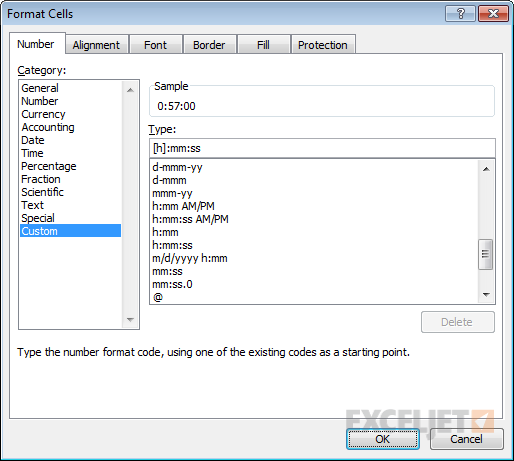
These are the number formats used in the example shown:
mm:ss // split times
h:mm:ss // total time
If total times may exceed 24 hours, use enclose the “h” in square brackets like “[h]”:
[h]:mm:ss
The square brackets tell Excel not to “reset” durations greater than 24 hours back to zero. Without the brackets, a time like 30:00:00 (30 hours) will display as 6:00:00 because Excel will reset the time to zero at 24 hours.
Tracking time with more precision
In the example above, we are tracking time down to a second, but there are cases where you will need to record time to a hundredth of a second or even a thousandth of a second (a millisecond). In that case, you will need to adjust the custom time format before entering the times. To enter time down to a hundredth of a second, use a custom time format like this:
mm:ss.00
To enter time down to a thousandth of a second (i.e. a millisecond), use a custom time format like this:
mm:ss.000
You will need to enter the seconds with a decimal value when a value is present. You can add h or [h] if needed to handle hours.
