Explanation
In this example, the goal is to sum by group, where each group is represented by a different color: Blue, Red, Green, and Purple. The worksheet shown contains two different approaches. In the range F5:G8, we have created a summary table to summarize counts by color. In column D, we are using a modified formula that reports a total per group the first time the group appears in the data. The article below explains both approaches.
Note: both formulas below use full column references (e.g. B:B, C:C). Full column references are a compact way to express a formula, and they automatically pick up new data in a column. However, they can also cause performance problems in some formulas, and they can return incorrect results when they intersect data elsewhere in a worksheet . In general, an Excel Table or a dynamic named range is a safer way to refer to data that may shrink or grow. All that said, you will run into full column references in worksheets developed by others, so it is important to understand how they work.
Summary table
One approach to solving this problem is to create a summary table to summarize results by group, as seen in the range F5:G8. The solution relies on the SUMIF function . The formula in G5, copied down, is:
=SUMIF(B:B,F5,C:C)
In this formula, B:B is the range , F5 is the criteria , and C:C is the sum_range . As the formula is copied down the column, the reference to F5 changes at each new row while the full column references do not change. The result is a subtotal by group of the amounts in column C.
Note: in the latest version of Excel, new functions make it possible to create summary tables that automatically update to include new groups. See this example for details.
Inline totals
Another way to approach this problem is to perform the calculations directly in the data in column D as seen in the worksheet. The formula in cell D5, copied down, is:
=IF(B5=B4,"",SUMIF(B:B,B5,C:C))
In this formula, we use the IF function to test each value in column B to see if its the same as the previous value (i.e. the cell above). If the two values match, we return an empty string (""). If the values do not match, the IF function returns this SUMIF formula:
SUMIF(B:B,B5,C:C)
This formula works the same way as the formula used in the summary table. As the formula is copied down the column, the reference to B5 changes at each new row while the full column references do not change. Because the IF function is suppressing the SUMIF formula when the values in column B match, the sums only appear in column D the first time a new color is encountered.
Note: this formula depends on data being sorted by group in order to get sensible results. One advantage of the summary table approach is that the sort order doesn’t matter.
Performance
As mentioned earlier, full column references can cause performance problems in some cases, because worksheets in Excel contain more than 1 million rows. Excel does try to limit calculations to the “used range” of a worksheet, in order to reduce the number of calculations being performed. However, be aware that full column references can cause severe performance problems in specific circumstances. Charles Williams over at Fast Excel has a good article on this topic, with a full set of timing results.
Why about Pivot Tables?
Pivot tables remain an excellent way to group and summarize data .
Explanation
In this example, the goal is to sum the amounts shown in column C by month using the dates in column B. The article below explains two approaches. One approach is based on the SUMIFS function , which can sum numeric values based on multiple criteria. The second approach is based on the SUMPRODUCT function , which allows a more flexible solution. For convenience, both solutions use the named ranges amount (C5:C16) and date (B5:B16).
Note: the values in E5:E10 are valid Excel dates , formatted to display the month name only with the number format “mmm”. See below for more information.
SUMIFS solution
The SUMIFS function can sum values in ranges based on multiple criteria. The syntax for SUMIFS looks like this:
=SUMIFS(sum_range,range1,criteria1,range2,criteria2,...)
In this problem, we need to configure SUMIFS to sum values by month using two criteria: one for a start date, and one for an end date. We start off with the sum_range , which contains the values to sum in amount (C5:C16):
=SUMIFS(amount,
To enter a criteria for the start date, we use the named range date (B5:B16) followed by a greater than or equal to operator (>=) concatenated to cell E5:
=SUMIFS(amount,date,">="&E5,
This works because cell E5 already contains the first day of the month, formatted to display the month only. To enter criteria for the end date, we use the EDATE function to advance one full month to the first day of the next month :
=EDATE(E5,1) // first of next month
We can then use the less than operator (<) to select the correct dates. The final formula in F5, copied down, is:
=SUMIFS(amount,date,">="&E5,date,"<"&EDATE(E5,1))
Roughly translated, the meaning of this formula is “Sum the amounts in C6:C16 when the date in B5:B16 is greater than or equal to the date in E5 and less than the first day of the next month”. Notice we need to concatenate the dates to logical operators , as required by the SUMIFS function. As the formula is copied down, it returns a total for each month in column E. The named ranges behave like absolute references and don’t change, while the reference to E5 is relative and changes at each new row.
Note: we could use the EOMONTH function to get the last day of the current month, then use “<=” as the second logical operator. However, because EOMONTH returns a date that is technically midnight, t here is a danger of excluding dates with times that occur on the last of the month. Using EDATE is a simpler and more robust solution.
With hardcoded dates
To use the SUMIFS function with hardcoded dates, the best approach is to use the DATE function like this:
=SUMIFS(amount,date,">="&DATE(2021,1,1),date,"<"&DATE(2021,2,1))
This formula uses the DATE function to create the first and last days of the month. This is a safer option than entering a date as text, because it guarantees that Excel will interpret the date correctly.
SUMPRODUCT option
Another nice way to sum by month is to use the SUMPRODUCT function together like this:
=SUMPRODUCT((TEXT(date,"mmyy")=TEXT(E5,"mmyy"))*amount)
In this version, we use the TEXT function to convert the dates to text strings in the format “mmyy”. Because there are 12 dates in the list, the result is an array with 12 values like this:
{"0122";"0222";"0222";"0322";"0322";"0322";"0422";"0422";"0422";"0522";"0522";"0522"}
Next, the TEXT function is used in the same way to extract the month and year from the date in E5:
TEXT(E5,"mmyy") // returns "0122"
The two results above are then compared to each other. The result is an array of TRUE and FALSE values like this:
{TRUE;FALSE;FALSE;FALSE;FALSE;FALSE;FALSE;FALSE;FALSE;FALSE;FALSE;FALSE}
This array indicates the dates in B5:B16 that are in the same month and year as the date in E5. The TRUE value in this array corresponds to the only date in January 2022. This array is then multiplied by the values in amount . The math operation automatically coerces the TRUE and FALSE values to 1s and 0s, so the final result inside SUMPRODUCT looks like this:
=SUMPRODUCT({100;0;0;0;0;0;0;0;0;0;0;0}) // returns 100
With just one array to process, the SUMPRODUCT sums the array and returns 100 as the result in F5. As the formula is copied down, the relative reference E5 changes at each new row, and SUMPRODUCT generates a new result. One nice feature of this formula is that it automatically ignores time values that may be attached to dates, so there is no need to worry about excluding datetimes that occur on the last day of the month, as with SUMIFS above.
Notes: (1) In the current version of Excel, which supports dynamic array formulas , you can substitute the SUM function for the SUMPRODUCT function. This article explains the details. (2) It would be nice to use the TEXT function inside the SUMIFS formula as well, but the SUMIFS function won’t accept an array operation in a range argument .
Display dates as names
To display the dates in E5:E10 as names only, you can apply the custom number format “mmmm”. Select the dates, then use Control + 1 to bring up the Format Cells Dialog box and apply the date format as shown below:
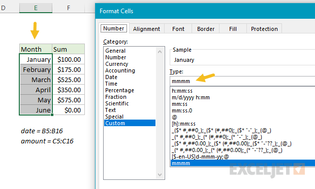
This allows you to use valid Excel dates in column E (required for the formula) and display them as you like.
Pivot Table solution
A pivot table is another excellent solution when you need to summarize data by year, month, quarter, and so on, because it can do this kind of grouping for you without any formulas at all. For a side-by-side comparison of formulas vs. pivot tables, see this video: Why pivot tables .
