Explanation
At the core, this formula relies on the SUMPRODUCT function to sum values in matching columns in the named range data C5:G14. If all data were provided to SUMPRODUCT in a single range, the result would be the sum of all values in the range:
=SUMPRODUCT(data) // all data, returns 387
To apply a filter by matching column headers – columns with headers that begin with “A” – we use the LEFT function like this:
LEFT(headers)=J4) // must begin with "a"
This expression returns TRUE if a column header begins with “a”, and FALSE if not. The result is an array:
{TRUE,TRUE,FALSE,FALSE,TRUE,FALSE}
You can see that values 1,2, and 5 correspond to columns that begin with “a”.
Inside SUMPRODUCT, this array is multiplied by “data”. Due to broadcasting , the result is a two-dimensional array like this:
{8,10,0,0,7,0;9,10,0,0,10,0;8,6,0,0,6,0;7,6,0,0,6,0;8,6,0,0,6,0;10,11,0,0,7,0;7,8,0,0,8,0;2,3,0,0,3,0;3,4,0,0,4,0;7,7,0,0,4,0}
If we visualize this array in a table, it’s easy to see that only values in columns that begin with “a” have survived the operation, all other columns are zero. In other words, the filter keeps values of interest and “cancels out” the rest:
| A001 | A002 | B001 | B002 | A003 | B003 |
|---|---|---|---|---|---|
| 8 | 10 | 0 | 0 | 7 | 0 |
| 9 | 10 | 0 | 0 | 10 | 0 |
| 8 | 6 | 0 | 0 | 6 | 0 |
| 7 | 6 | 0 | 0 | 6 | 0 |
| 8 | 6 | 0 | 0 | 6 | 0 |
| 10 | 11 | 0 | 0 | 7 | 0 |
| 7 | 8 | 0 | 0 | 8 | 0 |
| 2 | 3 | 0 | 0 | 3 | 0 |
| 3 | 4 | 0 | 0 | 4 | 0 |
| 7 | 7 | 0 | 0 | 4 | 0 |
With only a single array to process, SUMPRODUCT returns the sum of all values, 201.
Sum by exact match
The example above shows how to sum columns that begin with one or more specific characters. To sum column based on an exact match , you can use a simpler formula like this:
=SUMPRODUCT(data*(headers=J4))
FILTER function
In the latest version of Excel, you can solve this problem more directly with the FILTER function like this:
=SUM(FILTER(data,LEFT(headers)=J4,0))
In this formula, we use the same logic we used in the SUMPRODUCT function to select only data in columns that begin with the letter “A”:
LEFT(headers)=J4 // columns that begin with "A"
The expression above returns an array of TRUE and FALSE values like this:
{TRUE,TRUE,FALSE,FALSE,TRUE,FALSE}
Notice that the TRUE values correspond to column headers that begin with “A”. The FILTER function uses this array to select columns in the named range data . Because this array is horizontal , FILTER automatically filters on columns . The FILTER function returns the 3 columns in data with headers that begin with “A” to the SUM function, which returns a final result of 201.
Explanation
In this example, the goal is to sum values in matching columns and rows. Specifically, we want to sum values in data (C5:G14) where the column code is “A” and the day is “Wed”. One way to solve this problem is with the SUMPRODUCT function , which can handle array operations natively, without requiring control shift enter. In the latest version of Excel, the FILTER function is another option. Both approaches are explained below.
SUMPRODUCT function
In the example shown, the formula in J6 is:
=SUMPRODUCT((codes=J4)*(days=J5)*data)
where data (C5:G14), days (B5:B14), and codes (C4:G4) are named ranges . In this case, we are multiplying all values in the named range data by two expressions that “zero out” values that should not be included in the final sum:
(codes=J4)*(days=J5)
The first expression applies a condition based on codes:
(codes=J4)
Since J4 contains “B”, the expression creates an array of TRUE FALSE values like this:
{FALSE,TRUE,FALSE,TRUE,FALSE}
Each TRUE indicates a column where the code is “B”. The second expression tests for day:
(days=J5)
Since J4 contains “Wed”, the expression returns an array of TRUE and FALSE values like this:
{FALSE;FALSE;TRUE;FALSE;FALSE;FALSE;FALSE;TRUE;FALSE;FALSE}
In this array, each TRUE represents a row where the day in column B is “Wed”.
Next, the two arrays are multiplied together. In Excel, TRUE and FALSE values are automatically coerced to 1s and 0s by any math operation, so the multiplication step converts the arrays above to ones and zeros. When the horizontal array from the first expression is multiplied by the vertical array from the second expression, the result is a single two-dimensional array with the same dimensions as the original data:
{0,0,0,0,0;0,0,0,0,0;0,1,0,1,0;0,0,0,0,0;0,0,0,0,0;0,0,0,0,0;0,0,0,0,0;0,1,0,1,0;0,0,0,0,0;0,0,0,0,0}
The array above is 10 rows by 5 columns.The semi-colons (;) indicate rows, and the commas (,) indicate columns . When this array is multiplied by data , the operation effectively “zeros out” the values in data that should not be included in the final sum. The process can be visualized as shown below, where the “Filter array” is the array of 1s and 0s above.
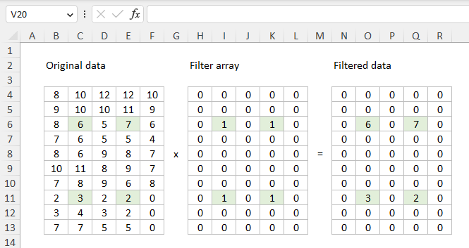
After data is multiplied by the Boolean array above, the result is a single array like this:
=SUMPRODUCT({0,0,0,0,0;0,0,0,0,0;0,6,0,7,0;0,0,0,0,0;0,0,0,0,0;0,0,0,0,0;0,0,0,0,0;0,3,0,2,0;0,0,0,0,0;0,0,0,0,0})
With just one array to process, SUMPRODUCT returns the sum of all elements in the final array, 18.
FILTER function
In the latest version of Excel, you can also use the FILTER function to solve this problem.
=SUM(FILTER(FILTER(data,codes=J4,0),days=J5,0))
This formula works in two steps. First, the inner FILTER returns columns where code is “B”:
FILTER(data,codes=J4,0) // filter columns
The resulting array is returned to the outer FILTER function, which returns rows where day is “Wed”:
=SUM(FILTER(array,days=J5,0)) // filter rows
The outer FILTER then returns matching data to the SUM function :
=SUM({6,7;3,2}) // returns 18
The SUM function then calculates a sum and returns a final result, 18.
Notes
- If you only need to sum matching columns (not rows) you can use a formula like this .
- To sum matching rows only, you can use the SUMIFS function .
