Explanation
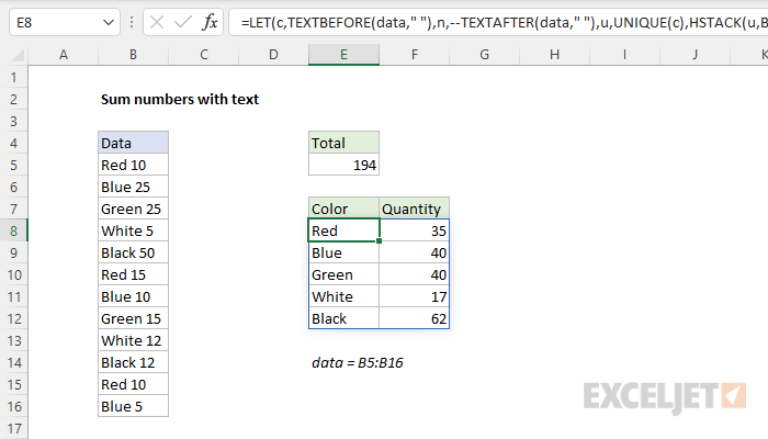
In this example, one goal is to sum the numbers that appear in the range B5:B16. A second more challenging goal is to create the table of results seen in E7:F12. For convenience, data is the named range B5:B16.
Total sum
To sum all the numbers that appear in B5:B16, ignoring text, the formula in E5 is:
=SUM(--TEXTAFTER(data," "))
Working from the inside out, the TEXTAFTER function is used to extract the numbers like this:
TEXTAFTER(data," ") // get all numbers
TEXTAFTER is configured to extract the text that occurs after a single space character (" “). Because we are giving TEXTAFTER 12 separate text strings in data (B5:B16), TEXTAFTER returns 12 results in an array like this:
{"10";"25";"25";"5";"50";"15";"10";"15";"12";"12";"10";"5"}
Notice that at this point the numbers are still text, as you can see by the double quotes (”). To coerce these text strings into actual numbers, we use a double negative (–):
--{"10";"25";"25";"5";"50";"15";"10";"15";"12";"12";"10";"5"}
The result is an array that contains numbers only:
{10;25;25;5;50;15;10;15;12;12;10;5}
This array is returned directly to the SUM function:
=SUM({10;25;25;5;50;15;10;15;12;12;10;5}) // returns 194
SUM returns 194 as the final result.
Summary table in two parts
One easy way to create the summary table seen in the worksheet is to use two formulas, one to list unique colors, and one to sum the numbers associated with each color. To list the unique colors starting in cell E8, you can use:
=UNIQUE(TEXTBEFORE(B5:B16," ")) // unique colors
This is a variation of the formula explained above. Instead of using TEXTAFTER, we are using the TEXTBEFORE function to get the text before the space (" “):
TEXTBEFORE(B5:B16," ") // get all colors
TEXTBEFORE returns an array of 12 colors like this:
{"Red";"Blue";"Green";"White";"Black";"Red";"Blue";"Green";"White";"Black";"Red";"Blue"}
This array is returned directly to the UNIQUE function , which returns an array with 5 unique colors:
{"Red";"Blue";"Green";"White";"Black"}
The array is returned to cell E8, and spills into the range E8:E12.
To sum the numbers associated with each color in column F, you can enter this formula in cell F8 and copy it down:
=SUM((TEXTBEFORE(data," ")=E8)*TEXTAFTER(data," "))
Note: we can’t use the SUMIF function in this case (which would be easier) because we don’t have the colors without numbers in an actual range . Instead, the colors exist in an array returned by the TEXTBEFORE function. SUMIF requires a range for the range argument.
All-in-one summary table
To create an all-in-one summary table that lists the unique dates along with a count for each date, you can use an advanced formula like this:
LET(
    c, TEXTBEFORE(data, " "),
    n, --TEXTAFTER(data, " "),
    u, UNIQUE(c),
    HSTACK(
        u,
        BYROW(u, LAMBDA(x, SUM(--(c = x) * n)))
    )
This is how the formula looks in the worksheet:
This formula utilizes the same patterns used in the formulas explained above, but now we move into more advanced functions like LET, LAMBDA, and BYROW.
The LET function is used to assign intermediate results to named variables. First, we use TEXTBEFORE to separate the colors from the numbers and assign the result to c. We use TEXTAFTER to separate the numbers and assign the result to n. Then we feed c into UNIQUE (to get unique colors) and assign the result to u. Next, we use the HSTACK function to combine two arrays. Array1 is u (the unique colors), and array2 is generated with the BYROW function :
BYROW(u, LAMBDA(x, SUM(--(c = x) * n)))
BYROW loops through each unique color in u and runs a custom LAMBDA function to sum the numbers associated with each color:
LAMBDA(x, SUM(--(c = x) * n))
The sum is generated with boolean logic and the SUM function :
SUM(--(c = x) * n)
The first part of the expression checks all colors (c) against the current row (x), generating an array of TRUE and FALSE values:
--(c = x)
The double negative (–) converts the TRUE and FALSE values to 1s and 0s. This array is then multiplied by all numbers (n). The numbers that survive are associated with the current row color (x) and the other numbers are converted to zero. SUM then returns the result for that row.
Note: Technically, the double negative (–) operation is not needed above because the multiplication step will automatically coerce the TRUE and FALSE values to 1s and 0s. However, it does no harm and perhaps makes the pattern of this formula easier to understand. In addition, if you remove the multiplication step, the result will be a count of each color rather than a sum. So the double negative allows the count variation of the formula to work without further adjustment.
The final result from the BYROW is an array with 5 sums:
{35;40;40;17;62}
This array is returned to HSTACK as array2 . HSTACK joins array1 and array2 together horizontally, and returns a 2-column array as a final result.
Explanation
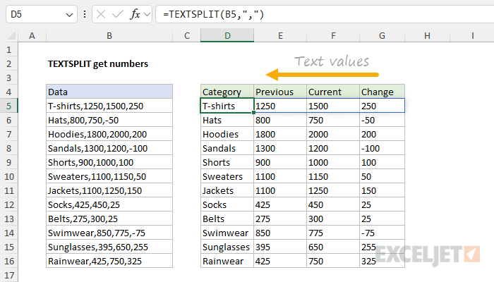
In this example, we have comma-separated text in column B. The goal is to split the text in column B into columns D through G while at the same time converting the numbers to true numeric values. The challenge is that TEXTSPLIT always returns text, so we need a way to convert the numbers while leaving the text values alone.
The problem with TEXTSPLIT
To split the text in column B into separate columns, we can use the TEXTSPLIT function with a simple formula like this:
TEXTSPLIT(B5,",")
This seems to work great. But the problem is that the numbers in columns E, F, and G aren’t really numeric values . Instead, they are text values, as you can see by the way Excel aligns them to the left:
If you use a function like SUM to sum these numbers up, the result will be zero . How can convert these numbers as text to actual numeric values? Well, one option is to use the VALUE function.
Adding the VALUE function
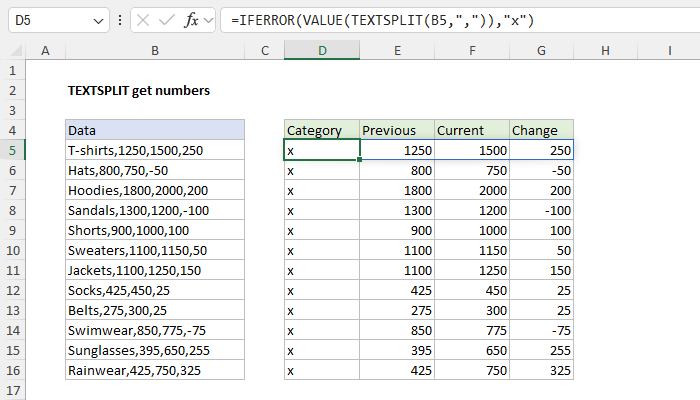
The VALUE function is designed to convert text that appears in a recognized format (i.e. a number, date, or time format) into a numeric value. If we wrap the VALUE function around the TEXTSPLIT function, this is the result:

Notice the numbers in columns E, F, and G are now actually numeric values, as we can see by the way Excel right-aligns them. However, we now have a new problem — the VALUE function has corrupted the text values in column D. This happens because when VALUE tries to convert the text to a number, the operation fails with a #VALUE! error. What we need is a way to selectively convert the “numbers as text” to numbers while leaving the text values alone. We can do that with the IFERROR function.
Adding the IFERROR function
The IFERROR function returns a custom result when a formula generates an error, and a standard result when no error is detected. The syntax for IFERROR looks like this:
=IFERROR(value,value_if_error)
To illustrate how this works, we can start by adding IFERROR like this:
=IFERROR(VALUE(TEXTSPLIT(B5,",")),"x")
Notice we have simply embedded the original formula above into IFERROR as the value argument, then provided the value “x” for value_if_error. The result looks like this:
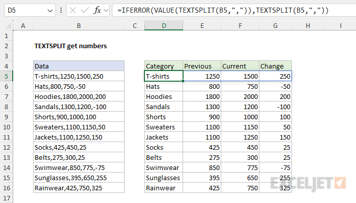
The “x” in column D tells us that IFERROR has encountered an error in this column, which is created when VALUE tries to convert the text values into numbers. The final step is to replace the “x” with the original text value. We can do that by simply repeating the original TEXTSPLIT formula. The final formula looks like this:
=IFERROR(VALUE(TEXTSPLIT(B5,",")),TEXTSPLIT(B5,","))
The result in the worksheet looks like this:
Optimizing with the LET function
The formula above works fine, but it would be inefficient with a large amount of data because we are running the same TEXTSPLIT operation twice. One way to improve performance is to use the LET function like this:
=LET(array,TEXTSPLIT(B5,","),IFERROR(VALUE(array),array))
In this formula, the result from TEXTSPLIT is assigned to a variable named “array”. We then use array inside the IFERROR and VALUE functions as above. The key difference is that TEXTSPLIT runs just one time .
