Explanation
Dates and times are just numbers in Excel, so you can use them in any normal math operation. However, by default, Excel will only display hours and minutes up to 24 hours. This means you might seem to “lose time” if you are adding up time that is more than 1 day.
In this example, the goal is to sum total hours in cell H5 and calculate total hours per person in the range H8:H10. All data is in an Excel Table named data in the range B5:E16. The table is used for convenience only, and is not required to solve the problem. The main challenge in this example is to correctly display time as a duration instead of time of day.
How Excel handles times
In Excel, dates are serial numbers and times are fractional parts of 1 day . This means the date and time values are just regular numbers and can be summed, added, and subtracted like other numbers. The screen below shows what the dates in column D and the times in column E look like with the General number format applied:

As you can see, dates are large serial numbers. The times in column E are just fractional values of one day, expressed as decimal values. This means you can use standard functions like SUM and SUMIF, etc. to sum time in various ways. But you have to be careful about how the result is displayed.
Excel times over 24 hours
What causes a time to look like a time in Excel is a number format . A simple number format for time might look like this:
h:mm // display time like 9:15
The main thing to understand is that a standard time format is meant to display time like a clock, which resets every 24 hours. This works fine when the goal is to display a time of day, or when total hours are less than 24. But in cases where time is meant to show a duration (i.e. elapsed time), the problem is that Excel will not display more than 24 hours by default. For example, if total time is 23 hours, the time format above will display “23:00”, but if total time is 31.5 hours, the time format above will display “7:30”:
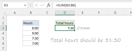
The time format causes hours to reset at midnight, and the extra 7.5 hours roll over into the next day. The formula is actually working fine, but the display makes it seem like hours are being undercounted or “lost” in the calculation.
Custom time format
To display 25 hours like “25:00”, we need to use a custom time format like this:
[h]:mm // display 25 hours as 25:00
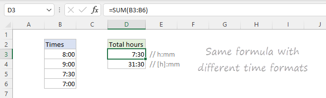
The square brackets around the “h” tell Excel to display hours as a duration, not a time of day. You can see how this works in the screen below. Cell D3 uses the time format “h:mm” and cell D4 uses the time format “[h]:mm”. Both cells contain the same formula:
=SUM(B3:B6)
Apply custom time format
To apply a custom time format, first select the cells you want to format and use Control + 1 to open the Format Cells window. Next, navigate to the Number tab, select Custom in the list to the left, and enter “[h]:mm” in the Type input area:

You will see a sample of the result displayed in the “Sample” area above Type.
Video: How to create a custom time format
Total time
With the above in mind, the formula to calculate total time in cell H5 is:
=SUM(data[Hours]) // sum all time
With the following custom time format above applied:
[h]:mm
The number returned by the SUM function is 3.1875 (3.19 days), which displays as 76:30 with the above time format applied.
Time per person
To calculate time logged per person, we use the SUMIF function . The formula in cell H8, copied down, is:
=SUMIF(data[Name],G8,data[Hours])
The range is the “Name” column of the table, the criteria is the value from G8 (“Jane”), and the sum_range is the “Hours” column. As the formula is copied down, SUMIF returns total hours per person. The range H8:H10 has the custom time format “[h]:mm” applied.
For more information on number formats, see Excel Custom Number formats.
Decimal time
Another solution for working with time values over 24 hours is to convert the time to a decimal number. For example, instead of using native time values like 4:30, 7:00, and 8:30, you convert these times to decimal hours like 4.5, 7.0, and 8.5. Once you have time in this format, you can calculate total time any way you like. This formula example explains the details.
Explanation
In this example, the sum range is the named range “time”, entered as an Excel time in hh:mm format. The first criteria inside SUMIFS includes dates that are greater than or equal to week date in column F:
date,">="&$F5
The second criteria limits dates to one week from the original date:
date,"<"&$F5+7
The last criteria, restricts data by project, by using the project identifier in row 4:
project,G$4
When this formula is copied across the range G5:H7, the SUMIFS function returns a sum of time by week and project. Notice all three criteria use mixed references to lock rows and columns as needed to allow copying.
Durations over 24 hours
To display time durations over 24 hours use a custom number format with hours in square brackets:
[h]:mm
