Purpose
Return value
Syntax
=SUMIFS(sum_range,range1,criteria1,[range2],[criteria2],...)
- sum_range - The range to be summed.
- range1 - The first range to evaluate.
- criteria1 - The criteria to use on range1.
- range2 - [optional] The second range to evaluate.
- criteria2 - [optional] The criteria to use on range2.
Using the SUMIFS function
The SUMIFS function sums numbers in Excel when they meet one or more specific conditions. SUMIFS is one of Excel’s most widely used functions, and you will see it in all kinds of spreadsheets that calculate conditional sums based on dates, text, or numbers. Although a common function, SUMIFS has a unique syntax that splits logical conditions into two parts, making it different from many other Excel functions. As a result, the task of defining criteria in SUMIFS can be a bit tricky. Also note that SUMIFS uses “AND logic”. To be included in the final result, all conditions must be TRUE.
Key features
- Sums values that meet one or more conditions
- Each new condition requires a separate range and criteria .
- Works with dates, text, and numbers
- Supports comparison operators (>, <, <>, =) and wildcards (*, ?)
- To be included in the final result, all conditions must be TRUE .
- All ranges must be the same size, or SUMIFS will return a #VALUE! error.
- Available in all Excel versions since Excel 2007
Unlike most other Excel functions, SUMIFS requires an actual range for sum/criteria ranges. If you try to use an array , Excel will not let you enter the formula. For details, see the example below .
- Syntax
- Basic Example
- Applying Criteria
- Criteria in another cell
- Not equal to
- Blank cells
- Dates
- Wildcards
- OR logic
- Summary Table
- Array Problem
- Limitations
- Notes
Syntax
The syntax for the SUMIFS function depends on the criteria being evaluated. Each condition is provided with a separate range and criteria . The generic syntax for SUMIFS looks like this:
=SUMIFS(sum_range,range1,criteria1) // 1 condition
=SUMIFS(sum_range,range1,criteria1,range2,criteria2) // 2 conditions
Note that the sum_range always comes first. This is the range of cells to sum. Each condition is provided as a pair of range/criteria arguments. The first formula above defines one condition and the second defines two. Additional conditions are defined by additional range/criteria pairs.
Basic Example
The worksheet below contains simple order data. We use SUMIFS to perform three calculations:
- Sum values where the color is Red.
- Sum values where the color is Red and the state is TX.
- Sum values where the color is Red, the state is TX, and the total is >20.
The three formulas in I5:I7 look like this:
=SUMIFS(F5:F16,C5:C16,"red") // Red
=SUMIFS(F5:F16,C5:C16,"red",D5:D16,"TX") // Red and TX
=SUMIFS(F5:F16,C5:C16,"red",D5:D16,"TX",F5:F16,">20") // Red and TX and >20

There are a few things worth noting in the formulas above:
- An equal sign (=) is not needed with “is equal to” criteria (i.e. use “red” not “=red”).
- SUMIFS is not case-sensitive, so “red” and “Red” will return the same results.
- Numbers must appear in quotes ("") when used with operators (i.e. “>20”).
- SUMIFS always uses “AND logic”. All conditions must be true.
Note that the syntax for the criteria argument in SUMIFS is somewhat unusual in Excel. Instead of simply entering >20 as the criteria, you must enter “>20” in double quotes. If you don’t quote values as required, Excel will not let you enter the formula . See below for more examples of this syntax.
Applying Criteria
The SUMIFS function supports logical operators (>,<,<>,=) and wildcards (*,?) for partial matching. The tricky part is the syntax needed to apply the criteria. This is because SUMIFS is in a group of eight functions that split logical criteria into two parts: range and criteria . Because of this design, operators must be enclosed in double quotes (""). The table below shows the syntax required for a variety of criteria:
| Target | Criteria |
|---|---|
| Cells greater than 75 | “>75” |
| Cells equal to 100 | 100 or “100” |
| Cells less than or equal to 100 | “<=100” |
| Cells equal to “Red” | “red” |
| Cells not equal to “Red” | “<>red” |
| Cells that are blank "" | "" |
| Cells that are not blank | “<>” |
| Cells that begin with “X” | “x*” |
| Cells equal to A1 | A1 |
| Cells less than A1 | “<"&A1 |
| Cells less than today | “<"&TODAY() |
Notice the last two examples involve concatenation with the ampersand (&) character. Any time you use a value from another cell or the result of a formula with a logical operator like “<”, you must concatenate. This is because Excel needs to evaluate cell references and formulas first before the value can used with an operator.
Criteria in another cell
It is often convenient to put criteria in another cell and then refer to this cell inside your formula. This makes it easy to change criteria later without editing the original formula. For example, you can sum cells in a range equal to the value in A1 like this:
=SUMIFS(sum_range,range,A1)
When a condition requires an operator, you must concatenate the cell reference to the operator. For example, to sum cells in a range greater than A1, use a formula like this:
=SUMIFS(sum_range,range,">"&A1)
Note we are joining the “>” operator to cell A1 with an ampersand (&) character. In the worksheet below, SUMIFS has been configured to return the sum of all sales over the value in G4. Notice the greater than operator (>), which is text, must be enclosed in quotes. The formula in G5 is:
=SUMIFS(D5:D9,D5:D9,">"&G4) // sum if greater than G4

Don’t enclose cell references in double quotes like “A1”. Doing so will convert them to text.
Not equal to
To express “not equal to” criteria, use the “<>” operator surrounded by double quotes (””). For example, use “<>red” for “not red”, and “<>blue” for “not blue”, as seen in the worksheet below:

=SUMIFS(C5:C9,B5:B9,"<>red") // not red
=SUMIFS(C5:C9,B5:B9,"<>blue") // not blue
=SUMIFS(C5:C9,B5:B9,"<>"&E7) // not E7
Note the following:
- In the last formula, we use E7 directly, so we need to concatenate like “<>"&E7.
- Do not use quotes around the cell reference.
- SUMIFS is not case-sensitive, so “red”, “RED”, and “Red” will return the same result.
Blank cells
SUMIFS can calculate sums based on whether cells are blank or not blank. Use an empty string (”") to target blank cells and the “not equal to” operator ("<>") to target cells that are not blank . In the worksheet below, SUMIFS is used to sum the amounts in column C depending on whether column D contains “x” or is empty:

=SUMIFS(C5:C9,D5:D9,"") // blank
=SUMIFS(C5:C9,D5:D9,"<>") // not blank
In the second formula, any value in a cell will cause SUMIFS to sum the amount. To be more precise, you can use a formula like this that sums values only when column D contains an “x”:
=SUMIFS(C5:C9,D5:D9,"x")
Dates
In Excel, dates are serial numbers , so you can use operators like <,>, <=, >= with dates like any other number. The tricky part about using dates in SUMIFS conditions is entering the dates in a way that Excel will understand. The most reliable way to do this is to refer to a valid date in another cell or use the DATE function . The example below shows both methods:

The formulas in F5:F8 are as follows:
=SUMIFS(C5:C12,B5:B12,"<"&DATE(2024,3,1))
=SUMIFS(C5:C12,B5:B12,">="&DATE(2024,3,31))
=SUMIFS(C5:C12,B5:B12,">"&E10)
=SUMIFS(C5:C12,B5:B12,">="&DATE(2024,5,1),B5:B12,"<="&DATE(2024,5,31))
Note the following:
- When using a cell reference, you must concatenate the reference to an operator like “>"&E10.
- In general, it’s best to avoid hardcoding a date into a formula and refer to a date in another cell instead.
- Referring to a date in another cell makes it easy to change the date without editing the formula.
Pro tip: Avoid hard-coding a date into a formula. Instead, put the date in a cell, then reference that cell in your formula. This makes the worksheet more useful since you can easily see the date being used and change the date when needed without editing the formula.
Wildcards
The SUMIFS function supports three wildcards you can use in criteria:
- Asterisk (*) - match zero or more characters
- Question mark (?) - match any one character
- Tilde (~) - an escape character to match a literal wildcard
The worksheet below shows how wildcards can be used with the SUMIFS function. The formulas in F5:F8 apply the criteria described in column E.
=SUMIFS(C5:C11,B5:B11,"mi*") // begins with "mi"
=SUMIFS(C5:C11,B5:B11,"*ota") // ends with "ota"
=SUMIFS(C5:C11,B5:B11,"????") // contains 4 characters
=SUMIFS(C5:C11,B5:B11,"*~?") // ends with "?"

Note the last formula in F8 uses “~?” to match a question mark (?) that occurs at the end of “Montana?” in cell C10. The tilde (~) is an escape character that allows you to find a literal wildcard. To match a question mark (?), use “~?”; to match an asterisk(), use “~*”; and to match a tilde (~), use “~~”. The table below shows more examples of how wildcards can be used:
| Pattern | Behavior | Will match |
|---|---|---|
| ? | Any one character | “A”, “B”, “c”, “z”, etc. |
| ?? | Any two characters | “AA”, “AZ”, “zz”, etc. |
| ??? | Any three characters | “Jet”, “AAA”, “ccc”, etc. |
| * | Any characters | “apple”, “APPLE”, “A100”, etc. |
| *th | Ends in “th” | “bath”, “fourth”, etc. |
| c* | Starts with “c” | “Cat”, “CAB”, “cindy”, “candy”, etc. |
| ?* | At least one character | “a”, “b”, “ab”, “ABCD”, etc. |
| ???-?? | Five characters with a hyphen | “ABC-99”,“100-ZT”, etc. |
| *~? | Ends with a question mark | “Hello?”, “Anybody home?”, etc. |
| xyz | Contains “xyz” | “code is XYZ”, “100-XYZ”, “XyZ90”, etc. |
Note: wildcards only work with text , not numbers.
OR logic
The SUMIFS function is designed to apply multiple conditions with “AND logic,” so there is no obvious way to sum cells with “OR logic”. However, one workaround is to provide the criteria as an array constant like {“red”,“blue}, and then nest the SUMIFS formula inside the SUM function like this:
=SUM(SUMIFS(sum_range,range,{"red","blue"})) // red or blue
The formula above will sum cells in sum_range when cells in range contain “red” or “blue”. Essentially, SUMIFS returns two sums, one for “red” and one for “blue”, and the SUM function returns the sum of the sums. For more details, see this example .
Summary Table
You can use SUMIFS to create a simple summary table. In the worksheet below, we have a list of unique colors in F5:F9. The goal is to subtotal the amounts in column D by color. The formula in cell G5, copied down, is:
=SUMIFS($D$5:$D$16,$C$5:$C$16,F5)

Notice that the range and the sum_range are locked as absolute references to prevent changes as the formula is copied down the column. If you are using Excel 2021 or later, you can generate all totals at once with a dynamic array formula like this:
=SUMIFS(D5:D16,C5:C16,F5:F9)
We don’t need the absolute references in this case because a single formula creates all results. You can go one step further by using the UNIQUE function in cell F5 to get a list of unique colors, then referring to the spill range directly like this:
=SUMIFS(D5:D16,C5:C16,F5#)
In Excel 365, you can also use the new GROUPBY function to create a summary table.
Array Problem
Note: For more advanced use cases, this is an important limitation in what SUMIFS can do.
One of the more tricky limitations of SUMIFS is that it won’t allow an array for a range argument. To understand the problem, consider the worksheet below, where we have 12 dates in column B and 12 amounts in column C. The goal is to create a formula to sum the amounts by year. We can do that with the following SUMIFS formula:
=SUMIFS(C5:C16,B5:B16,">="&DATE(E5,1,1),B5:B16,"<="&DATE(E5,12,31))
Note: I would normally use absolute references for the two ranges so that the formula can be copied down without changes, but I have left the addresses relative here so they are easier to read.

This formula works fine, but it’s a little complicated. If you have some experience with Excel formulas, you might think you can use SUMIFS and YEAR together in a clever formula like this:
=SUMIFS(C5:C16,YEAR(B5:B16),E5)
The idea is to extract the year from the dates in column B with the YEAR function , and then use 2024 (in cell E5) for the criteria. This would be cool if it worked. However, Excel won’t even let you enter this formula. If you try, you’ll get a generic “There’s a problem with your formula” error:

The problem is that SUMIFS requires a proper range for the range argument, but YEAR(B5:B16) will return an array like this:
{2024;2024;2024;2024;2024;2025;2025;2025;2025;2025;2025;2025}
To be clear, using YEAR like this works fine in most other formulas. However, SUMIFS is not programmed to handle arrays, so it won’t work. How can we work around this problem? One nice alternative is to switch to the SUMPRODUCT function and use a formula like this:
=SUMPRODUCT(sum_range,--(range=criteria))
If we modify the pattern above to fit the workbook example, we get the following:
=SUMPRODUCT(C5:C16,--(YEAR(B5:B16)=E5))
This formula is quite a bit simpler than the SUMIFS formula above. It’s a good example of how SUMPRODUCT can often solve a tricky problem in a clever and elegant formula.
Remember: If you try to provide an array for a range, you won’t be able to enter the formula because Excel will display a “There’s a problem with your formula” error dialog. The “array problem” is not mentioned explicitly.
Limitations
The SUMIFS function has several limitations you should be aware of:
- Conditions in SUMIFS are joined by AND logic. In other words, all conditions must be TRUE in order for a cell to be included in a sum. To sum cells with OR logic, you can use a workaround in simple cases.
- All ranges must be the same size. If you supply ranges that don’t match, you’ll get a #VALUE error. See example here .
- The SUMIFS function requires actual ranges for all range arguments; you can’t use an array . This means you can’t do things like extract the year from dates inside the SUMIFS function. To alter values that appear in a range argument before applying criteria, the SUMPRODUCT function is a flexible solution.
- SUMIFS is not case-sensitive. To sum values based on a case-sensitive condition, you can use a formula based on the SUMPRODUCT function with the EXACT function .
- If you reference a range in an external workbook, SUMIFS requires that the workbook be open to calculate a result. If the external workbook is not open, you will see a #VALUE! error. As a workaround, you can switch to the SUMPRODUCT function, which does not have this limitation. The syntax will look like this: =SUMPRODUCT(–(criteria_range1=criteria1), –(criteria_range2=criteria2) … , sum_range). See this page for details.
- SUMIFS has some other quirks, which are detailed in this article .
The most common way to work around most of these limitations is to use the SUMPRODUCT function .
Notes
- Multiple conditions are applied using AND logic, i.e., condition 1 AND condition 2, etc.
- All ranges must be the same size. If you supply ranges that don’t match, you’ll get a #VALUE error.
- Non-numeric criteria must be enclosed in double quotes (i.e., “<100”, “>32”, “TX”).
- Cell references in criteria are not enclosed in quotes, i.e., “<"&A1
- The wildcard characters “?” and “” can be used in criteria. A question mark (?) matches any one character, and an asterisk () matches any sequence of characters (zero or more).
- To match a literal question mark(?) or asterisk (), use a tilde (~) like (~?, ~).
- SUMIFS requires a range ; you can’t substitute an array .
Purpose
Return value
Syntax
=SUMPRODUCT(array1,[array2],...)
- array1 - The first array or range to multiply, then add.
- array2 - [optional] The second array or range to multiply, then add.
Using the SUMPRODUCT function
The SUMPRODUCT function multiplies arrays together and returns the sum of products. If only one array is supplied, SUMPRODUCT will simply sum the items in the array. Up to 30 ranges or arrays can be supplied. When you first encounter SUMPRODUCT, it may seem boring, complex, and even pointless. But SUMPRODUCT is an amazingly versatile function with many uses. Because it will handle arrays gracefully, you can use it to process ranges of cells in clever, elegant ways.
Key features
Works with arrays natively in older versions of Excel (no need for Ctrl+Shift+Enter)
Can apply complex AND/OR logic using Boolean algebra
Works for conditional sums, counts, and averages (can replace SUMIFS, COUNTIFS, AVERAGEIFS)
Automatically treats non-numeric values as zeros (like the SUM function)
Can use other functions like LEN, ISBLANK, ISTEXT, ISERROR, etc., directly
Works in all Excel versions
Classic SUMPRODUCT example
SUMPRODUCT for conditional sums
SUMPRODUCT for conditional sums and counts
SUMPRODUCT with double negative (–)
SUMPRODUCT with OR logic
SUMPRODUCT with abbreviated syntax
Ignoring empty cells
SUMPRODUCT with other functions
Arrays and Excel 365
Classic SUMPRODUCT example
The “classic” SUMPRODUCT example illustrates how you can calculate a sum directly without a helper column . For example, in the worksheet below, you can use SUMPRODUCT to get the total of all numbers in column F without using column F at all:
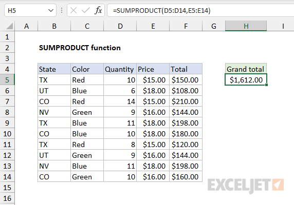
To perform this calculation, SUMPRODUCT uses values in columns D and E directly like this:
=SUMPRODUCT(D5:D14,E5:E14) // returns 1612
The result is the same as summing all values in column F. The formula is evaluated like this:
=SUMPRODUCT(D5:D14,E5:E14)
=SUMPRODUCT({10;6;14;9;11;10;8;9;11;10},{15;18;15;16;18;18;15;16;18;16})
=SUMPRODUCT({150;108;210;144;198;180;120;144;198;160})
=1612
This use of SUMPRODUCT can be handy, especially when there is no room (or need) for a helper column with an intermediate calculation. However, the most common use of SUMPRODUCT in the real world is to apply conditional logic in situations that require more flexibility than functions like SUMIFS and COUNTIFS can offer.
SUMPRODUCT for conditional sums
A typical use for the SUMPRODUCT function is to calculate conditional sums, much like you would use a function like SUMIFS. In the worksheet shown below, SUMPRODUCT is used to calculate conditional sums with four separate formulas:
=SUMPRODUCT(--(C5:C14="red"),F5:F14) // red
=SUMPRODUCT(--(B5:B14="tx"),--(C5:C14="red"),F5:F14) // tx and red
=SUMPRODUCT(--(B5:B14="co"),--(C5:C14="blue"),F5:F14) // co and blue
=SUMPRODUCT(--(C5:C14<>"red"),F5:F14) // not red
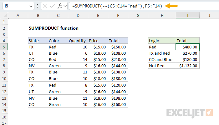
The results are visible in cells I5, I6, I7, and I8. The article below explains how SUMPRODUCT can be used to calculate these kinds of conditional sums, and the purpose of the double negative (–) in the formulas.
SUMPRODUCT for conditional sums and counts
The SUMPRODUCT function can be used for conditional sums or counts. To illustrate how this works, let’s look at a very simple example. Assume we have some order data in A2:B6, with State in column A, and Sales in column B:
| A | B | |
|---|---|---|
| 1 | State | Sales |
| 2 | UT | 75 |
| 3 | CO | 100 |
| 4 | TX | 125 |
| 5 | CO | 125 |
| 6 | TX | 150 |
Using SUMPRODUCT, you can sum total sales for Texas (“TX”) with this formula:
=SUMPRODUCT(--(A2:A6="TX"),B2:B6)
You can also count total sales for Texas (“TX”) with this formula:
=SUMPRODUCT(--(A2:A6="TX"))
Notice we have retained the conditional logic –(A2:A6=“TX”) from the formula above, and simply removed the second array (Sales). This is the basic idea of counting with SUMPRODUCT. The conditional logic remains, but the second array is removed. However, to make this work, we need a way to coerce the true and false values that the logic creates into ones and zeros. Let’s look at that next.
SUMPRODUCT with double negative (–)
The formulas above use a double negative (–) to make the conditional logic work properly. To understand why this is necessary, let’s trace through exactly what happens when SUMPRODUCT processes our Texas example. When Excel evaluates the expression A2:A6=“TX” , it creates an array of TRUE and FALSE values based on which cells match “TX”. Here’s what the two arrays look like initially:
| array1 | array2 | Product | Result |
|---|---|---|---|
| FALSE | 75 | FALSE * 75 | 0 |
| FALSE | 100 | FALSE * 100 | 0 |
| TRUE | 125 | TRUE * 125 | 0 |
| FALSE | 125 | FALSE * 125 | 0 |
| TRUE | 150 | TRUE * 150 | 0 |
| Sum | 0 |
Array1 contains the TRUE/FALSE results from our condition, while array2 contains the corresponding sales values. The problem is that SUMPRODUCT needs to multiply these arrays together, but the raw TRUE and FALSE values can’t be used directly because they are treated as zeros, making our entire calculation return zero.
This is where the double negative becomes important. The double negative is one of several ways to convert TRUE and FALSE values into their numeric equivalents: TRUE becomes 1, and FALSE becomes 0. This conversion enables Boolean logic operations within our formula. After applying the double negative, here’s how the table above works:
| array1 | array2 | Product | ||
|---|---|---|---|---|
| 0 | * | 75 | = | 0 |
| 0 | * | 100 | = | 0 |
| 1 | * | 125 | = | 125 |
| 0 | * | 125 | = | 0 |
| 1 | * | 150 | = | 150 |
| Sum | 275 |
Now SUMPRODUCT can perform the calculation successfully. In array terms, the formula evaluates like this:
=SUMPRODUCT({0,0,1,0,1},{75,100,125,125,150})
SUMPRODUCT multiplies the corresponding elements of both arrays, then sums the result:
=SUMPRODUCT({0,0,125,0,150}) // returns 275
The same double negative principle applies to our conditional count example. Recall that we can count Texas sales using =SUMPRODUCT(–(A2:A6=“TX”)) . After applying the double negative, we get the array {0,0,1,0,1} . Since we’re only providing one array to SUMPRODUCT (no second array to multiply against), SUMPRODUCT simply sums the values in this single array: 0+0+1+0+1 = 2. This gives us a count of 2, representing the two rows where the state equals “TX”. The double negative is essential here because without it, SUMPRODUCT would receive {FALSE,FALSE,TRUE,FALSE,TRUE} and treat these logical values as zeros, returning 0 instead of the correct count.
This example expands on the ideas above with more detail.
SUMPRODUCT with OR logic
It is also possible to use the SUMPRODUCT function with OR logic, i.e., sum if this or that. The trick is to use Boolean logic, where OR logic is represented with addition (+). You can see this approach in the worksheet below:

The formulas in I5:I7 are as follows:
=SUMPRODUCT(--((C5:C14="red")+(C5:C14="blue")>0),F5:F14) // red or blue
=SUMPRODUCT(--((B5:B14="tx")+(C5:C14="red")>0),F5:F14) // tx or red
=SUMPRODUCT(--((B5:B14="co")+(C5:C14="blue")>0),F5:F14) // co or blue
Notice that the two logical expressions are joined with addition (+), and the resulting array is checked against zero (>0) and then converted to 1s and 0s with the double negative (–):
--((C5:C14="red")+(C5:C14="blue")>0)
For a more detailed explanation of how and why this works, watch this 3-minute video: Boolean algebra in Excel . Also, see this example , which explains several ways to approach a problem like this.
SUMPRODUCT with abbreviated syntax
You will often see the formula described above written in a different way, like this:
=SUMPRODUCT((A2:A6="TX")*B2:B6) // returns 275
Notice that all calculations have been moved into array1 . The result is the same, but this syntax provides several advantages. First, the formula is more compact, especially as the logic becomes more complex. This is because the double negative (–) is no longer needed to convert TRUE and FALSE values — the math operation of multiplication ( ) automatically converts the TRUE and FALSE values from (A2:A6=“TX”) to 1s and 0s. But the most important advantage is flexibility . When using separate arguments, the operation is always multiplication, since SUMPRODUCT returns the sum of products*. This limits the formula to AND logic since multiplication corresponds to addition in Boolean algebra . Moving calculations into one argument means you can use addition (+) for OR logic, in any combination. In other words, you can choose your own math operations, which ultimately dictate the logic of the formula. See example here .
Even though the double negative is no longer needed, there is no harm in leaving it in the formula.
With the above advantages in mind, there is one disadvantage to the abbreviated syntax. SUMPRODUCT is programmed to ignore the errors that result from multiplying text values in arrays given as separate arguments . This can be handy in certain situations . With the abbreviated syntax, this advantage goes away, since the multiplication happens inside a single array argument. In this case, the normal behavior applies: text values will create #VALUE! errors.
Note: Technically, moving calculations into array1 creates an " array operation “, and SUMPRODUCT is one of only a few functions that can handle an array operation natively without Control + Shift + Enter in Legacy Excel . See Why SUMPRODUCT? for more details.
Ignoring empty cells
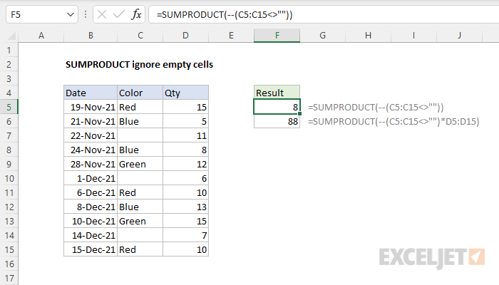
To ignore empty cells with SUMPRODUCT, you can use an expression like range<>”” . In the example below, the formulas in F5 and F6 both ignore cells in column C that do not contain a value:
=SUMPRODUCT(--(C5:C15<>"")) // count
=SUMPRODUCT(--(C5:C15<>"")*D5:D15) // sum
SUMPRODUCT with other functions
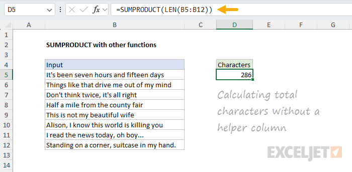
SUMPRODUCT can use other functions directly. You might see SUMPRODUCT used with the LEN function to count total characters in a range, or with functions like ISBLANK, ISTEXT, etc., to count blanks in a range or text values in a range. These are not normally array functions, but when they are given a range, they create an array of results. Because SUMPRODUCT is built to work with arrays, it is able to perform calculations on the arrays directly. You can see an example of this in the worksheet below, where we have eight text strings in the range B5:B12, and we are using SUMPRODUCT with the LEN function to calculate the total characters in the range with this formula in cell D5:
=SUMPRODUCT(LEN(B5:B12))
For example, assume you have 10 different text values in A1:A10 and you want to count the total characters for all 10 values. You could add a helper column in column B that uses this formula: LEN(A1) to calculate the characters in each cell. Then you could use SUM to add up all 10 numbers. However, using SUMPRODUCT, you can write a formula like this:
=SUMPRODUCT(LEN(A1:A10))
Working from the inside out, the LEN function runs first and returns an array of 8 results. The SUMPRODUCT function then sums the array and returns the final result. The formula evaluates like this:
=SUMPRODUCT(LEN(A1:A10))
=SUMPRODUCT({38;40;33;32;29;40;32;42})
=286
The final result is 286. To be clear, you can use the SUM function to do the same thing in a current version of Excel. However, in older versions of Excel (Excel 2019 and older), using SUMPRODUCT this way is a way to avoid having to enter the formula using Ctrl+Shift+Enter.
Arrays and Excel 365
This is a confusing topic, but it must be mentioned. In Excel 2019 and earlier, the SUMPRODUCT function can be used to create array formulas that don’t require Ctrl + Shift + Enter . This is a key reason that SUMPRODUCT was so widely used to create more advanced formulas for the past 20 years or so, up to the introduction of dynamic array formulas. Using SUMPRODUCT was a way to get array formulas to work in any version of Excel without special handling .
However, in Excel 365 , the formula engine handles arrays natively . This means you can often use the SUM function in place of SUMPRODUCT in an array formula with the same result, with no need to enter the formula in a special way. However, if the same formula is opened in an earlier version of Excel, it will still require Ctrl + Shift + Enter to work correctly .
The bottom line is that SUMPRODUCT is a safer option if a worksheet will be used often in older versions of Excel. For more details and examples, see Why SUMPRODUCT?
Notes
- SUMPRODUCT treats non-numeric items in arrays as zeros.
- Array arguments must be the same size. Otherwise, SUMPRODUCT will generate a #VALUE! error value.
- Logical tests inside arrays will create TRUE and FALSE values. In most cases, you’ll want to coerce these to 1’s and 0’s.
- SUMPRODUCT can often use the result of other functions directly.
