Explanation
The SUMPRODUCT function multiplies arrays together and returns the sum of products. If only one array is supplied, SUMPRODUCT will simply sum the items in the array. For example, if we give SUMPRODUCT one array in the form of the data[Qty] column:
=SUMPRODUCT(data[Qty]) // returns 54
SUMPRODUCT returns 54, the total of all numbers in the Qty column, like this:
=SUMPRODUCT(data[Qty])
=SUMPRODUCT({9;6;4;8;5;1;7;5;4;2;3})
=54
What we need now is a way to “filter” these values to include only the value associated with “Red”, respecting case. In other words, we need to test the values in the Color column and only allow those associated with “Red” to make it through. We can do this with the EXACT function , which is designed to perform a case-sensitive comparison of text strings. We use EXACT like this:
--EXACT(F5,data[Color])
Because we are comparing the in value in F5 (“Red”) with the eleven values in the Color column, the EXACT function returns 11 results in an array like this:
{FALSE;FALSE;FALSE;FALSE;TRUE;FALSE;FALSE;FALSE;FALSE;FALSE;FALSE}
Next, we use a double negative (–) in front of EXACT to convert the TRUE and FALSE values to 1s and 0s. The resulting array looks like this:
{0;0;0;0;1;0;0;0;0;0;0}
Notice the 1 in the 5th position corresponds to the “Red” in row 5. Every other value is now a zero. This will work perfectly as a filter. Turning back to the formula in G5, we can see how this works. The formula is evaluated like this:
=SUMPRODUCT(--EXACT(F5,data[Color]),data[Qty])
=SUMPRODUCT({0;0;0;0;1;0;0;0;0;0;0},{9;6;4;8;5;1;7;5;4;2;3})
=SUMPRODUCT({0;0;0;0;5;0;0;0;0;0;0})
=5
Each array is evaluated, the two arrays are multiplied together, and SUMPRODUCT returns the sum of the products. The FALSE values created with the EXACT function become zeros, and the zeros effectively cancel out the other values when the two arrays are multiplied together. The only values that survive are those associated with TRUE, and the final result is 5.
Remember, this formula only works for numeric values, because SUMPRODUCT doesn’t handle text.
Case-sensitive sum
Note that because we are using SUMPRODUCT, this formula comes with a unique twist: if there are multiple matches, SUMPRODUCT will return the sum of those matches. For example, the value in cell F6 is “RED”, which appears twice in the Color column. The formula in G6 returns 9 like this:
=SUMPRODUCT(--EXACT(F6,data[Color]),data[Qty])
=SUMPRODUCT({0;0;1;0;0;0;0;1;0;0;0}*{9;6;4;8;5;1;7;5;4;2;3})
=SUMPRODUCT({0;0;4;0;0;0;0;5;0;0;0}) // returns 9
The value “RED” appears in row 3 and row 8 of the table, and the final sum is 9.
Compact syntax
In more advanced SUMPRODUCT formulas, you will often see an abbreviated syntax like this:
=SUMPRODUCT(EXACT(F6,data[Color])*data[Qty])
Notice we are now providing just one array to SUMPRODUCT, which is a result of multiplying the two arrays together directly. The advantage of this approach is that we no longer need to use the double negative. The math operation of multiplying the arrays together automatically coerces the TRUE and FALSE values in the first array into 1s and 0s.
Explanation
The goal is to lookup a feed rate based on material, hardness, and drill bit diameter. Feed rate values are in the named range data (D6:H16).
This can be done with a two-way INDEX and MATCH formula. One MATCH function works out the row number (material and hardness), and the other MATCH function finds the column number (diameter). The INDEX function returns the final result.
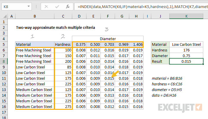
In the example shown, the formula in K8 is:
=INDEX(data,
MATCH(K6,IF(material=K5,hardness),1), // get row
MATCH(K7,diameter,1)) // get column
(Line breaks added for readability only).
The tricky bit is that material and hardness need to be handled together. We need to restrict MATCH to the hardness values for a given material (Low Carbon Steel in the example shown).
We can do this with the IF function. Essentially, we use IF to “throw away” irrelevant values before we look for a match.
Details
The INDEX function is given the named range data (D6:H16) as for array. The first MATCH function works out the row number:
MATCH(K6,IF(material=K5,hardness),1) // get row num
To locate the correct row, we need to do an exact match on material, and an approximate match on hardness. We do this by using the IF function to first filter out irrelevant hardness:
IF(material=K5,hardness) // filter
We test all of the values in material (B6:B16) to see if they match the value in K5 (“Low Carbon Steel”). If so, the hardness value is passed through. If not, IF returns FALSE. The result is an array like this:
{FALSE;FALSE;FALSE;85;125;175;225;FALSE;FALSE;FALSE;FALSE}
Notice the only surviving values are those associated with Low Carbon Steel. The other values are now FALSE. This array is returned directly to the MATCH function as the lookup_array.
The lookup value for match comes from K6, which contains the given hardness, 176. MATCH is configured for approximate match by setting match_type to 1. With these settings, MATCH ignores FALSE values and returns the position of an exact match or the next smallest value.
Note: hardness values must be sorted in ascending order for each material.
With hardness given as 176, MATCH returns 6, delivered directly to INDEX as the row number. We can now rewrite the original formula like this:
=INDEX(data,6,MATCH(K7,diameter,1))
The second MATCH formula finds the correct column number by performing an approximate match on diameter:
MATCH(K7,diameter,1) // get column num
Note: values in diameter D5:H5 must be sorted in ascending order.
The lookup value comes from K7 (0.75), and the lookup_array is the named range diameter (D5:H5).
As before, the MATCH is set to approximate match by setting match_type to 1.
With diameter given as 0.75, MATCH returns 3, delivered directly to the INDEX function as the column number. The original formula now resolves to:
=INDEX(data,6,3) // returns 0.015
INDEX returns a final result of 0.015, the value from F11.
