Explanation
In this example, the goal is to count rows where the value in column one is “A” or “B” and the value in column two is “X”, “Y”, or “Z”. In the worksheet shown, we are using array constants to hold the values of interest, but the article also shows how to use cell references instead. In simple scenarios, you can use Boolean logic and the addition operator (+) to count with OR logic , but as the number of values being testing increases, the formula becomes unwieldy. To keep the formula as tidy as possible, this example uses the MATCH function together with the ISNUMBER function to check more than one value at a time.
ISNUMBER + MATCH
Working from the inside out, each condition is applied with a separate ISNUMBER + MATCH expression. To generate a count of rows in column one where the value is A or B we use the following code:
ISNUMBER(MATCH(B5:B11,{"A","B"},0)
Notice the values “A” and “B” are supplied as an array constant and match_type is set to zero for an exact match.
Note: the configuration for MATCH may appear “reversed” from what you might expect. This is necessary in order to preserve the structure of the source data in the results returned by MATCH, i.e. we get back seven results, one for each row in B5:B11.
Since we give the MATCH function 7 values to look for, MATCH returns an array that contains 7 results like this:
{1;2;#N/A;1;2;1;2}
Each number in this array represents a match on “A” or “B” in Column B (1=“A”, 2=“B”). An #N/A error indicates a row where neither value was found. These results are delivered directly to the ISNUMBER function , which is used to convert the values from MATCH into simple TRUE and FALSE results:
ISNUMBER({1;2;#N/A;1;2;1;2})
ISNUMBER returns a new array that looks like this:
{TRUE;TRUE;FALSE;TRUE;TRUE;TRUE;TRUE}
In this array, TRUE values represent rows where “A” or “B” were found in column B. The next step is to test for “X”,“Y”,or “Z” in column C, and for this we use exactly the same approach:
ISNUMBER(MATCH(C5:C11,{"X","Y","Z"},0))
With the above configuration, the MATCH function returns the following array:
{1;2;3;3;#N/A;1;2}
As before, the ISNUMBER function converts these results to TRUE and FALSE values and returns an array like this:
{TRUE;TRUE;TRUE;TRUE;FALSE;TRUE;TRUE}
We now have everything we need to perform the count, and for this we use the SUMPRODUCT function.
SUMPRODUCT function
The final step in the formula is to tally up the rows that meet the criteria outlined above. In the example shown, the formula in F10 is:
=SUMPRODUCT(ISNUMBER(MATCH(B5:B11,{"A","B"},0))*
ISNUMBER(MATCH(C5:C11,{"X","Y","Z"},0)))
After the two MATCH and ISNUMBER expressions are evaluated, the formula simplifies to the following:
=SUMPRODUCT({TRUE;TRUE;FALSE;TRUE;TRUE;TRUE;TRUE}*{TRUE;TRUE;TRUE;TRUE;FALSE;TRUE;TRUE})
Next, the two arrays are multiplied together inside SUMPRODUCT, which automatically converts TRUE FALSE values to 1s and 0s as a result of the math operation:
=SUMPRODUCT({1;1;0;1;1;1;1}*{1;1;1;1;0;1;1})
Once the two arrays are multiplied together, we have a single array like this:
=SUMPRODUCT({1;1;0;1;0;1;1}) // returns 5
In this array, a 1 signifies a row that meets all criteria and a 0 indicates a row that does not. With just a single array to process, SUMPRODUCT sums the array and returns a final result of 5.
With cell references
The example above uses hardcoded array constants, but you can also use cell references:
=SUMPRODUCT(ISNUMBER(MATCH(B5:B11,E5:E6,0))*ISNUMBER(MATCH(C5:C11,F5:F7,0)))
This approach can be “scaled up” to handle more criteria. You can see an example in this formula challenge .
Note: The SUMPRODUCT function is used below for compatibility with Legacy Excel . In the current version of Excel, you can use the SUM function instead. For more on this topic, see: Why SUMPRODUCT?
Explanation
In this example, the goal is to count the people shown in the table by both Department (Dept) and Group as shown in the worksheet. A simple way to do this is with the COUNTIFS function.
COUNTIFS function
The COUNTIFS function is designed to count things based on more than one condition. Conditions are supplied to COUNTIFS in range/criteria “pairs” like this:
=COUNTIFS(range1,criteria1,range2,criteria2)
In this problem, the first step is to create the shell of the summary table that contains one set of criteria in the left-most column, and the second set of criteria in the top row as column headers like this:

The next step is to enter the COUNTIFS function in cell G5 with the first condition for Department:
=COUNTIFS(dept,$F5
For criteria_range1 , we use the named range dept (B5:B16). For criteria1 , we use the mixed reference $F5. Cell F5 contains the value “Engineering”, which will be used for criteria. We use a mixed reference to lock the column only so that the formula will still refer to column F when we copy it to the next column. We leave the row relative because we want the row to change as we copy the formula down. Note that a named range automatically behaves like an absolute reference , so we don’t need to do anything special with the range; it will not change when copied.
Next, we enter the second range/criteria pair to target values for Group:
=COUNTIFS(dept,$F5,group,G$4)
For criteria_range2 , we use the named range group (C5:C16). For criteria2 , we use the mixed reference G$4. Cell G4 contains the value “A”, which will be used for criteria. We use a mixed reference to lock the row only so that the formula will still refer to row 4 when we copy it down.
This is the final formula entered in cell G5, and copied into the range G5:H8. To recap, the named ranges dept and group automatically behave like absolute references and will not change. The references to $F5 and G$4 however are mixed. As the formula is copied, the row in $F5 changes and the column in G$4 changes, which allows the COUNTIFS function to generate correct counts for all combinations of Department and Group.
Excel Table option
When you use an Excel Table to hold source data, you get some nice benefits, including a table that automatically expands when rows are added. Excel Tables use structured references , which appear automatically in formulas that refer to them. In the screen below, the formula in G5 is:
=COUNTIFS(data[[Dept]:[Dept]],$F5,data[[Group]:[Group]],G$4)
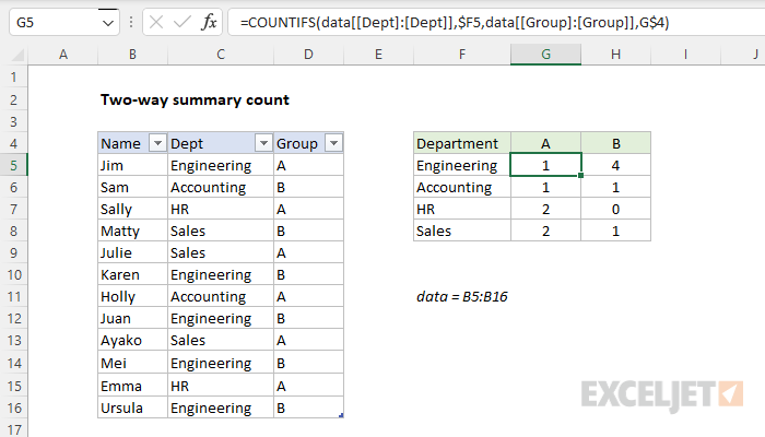
This formula is a bit more complex than usual, because the Dept and Group columns need to be locked in a special way with the double square brackets and a colon to allow the formula to be copied across the summary tabled. The two references below show this difference in syntax:
data[Dept] // normal
data[[Dept]:[Dept]] // locked
For more on Excel Tables and structured references, see the videos below. One of the videos shows an easy way to lock a structured reference. If you are new to Excel Tables, see What is an Excel Table ?
Dynamic array option
In the latest version of Excel, which supports dynamic array formulas , you can adapt this example to automatically extract the values for Dept and Group with the UNIQUE function . If fact, if we throw in the LET function and two new functions, HSTACK and VSTACK , it is possible to write a single all-in-one formula that builds a complete summary table like this:
=LET(
  depts,UNIQUE(data[Dept]),
  groups,TRANSPOSE(UNIQUE(data[Group])),
  counts,COUNTIFS(data[Dept],depts,data[Group],groups),
  HSTACK(VSTACK({"Department"},depts),VSTACK(groups,counts))
)
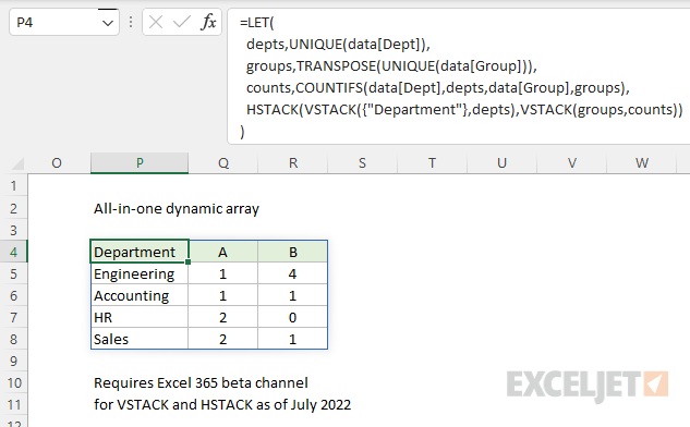
Note: VSTACK and HSTACK are still in beta, available via the Beta Channel for Excel 365.
The best thing about this approach is that any changes to the source data will be reflected in the summary table instantly, with no need to refresh or edit the formula. As a bonus, there is no need to lock specific cell references. The formula above is a great example of how dynamic array formulas will completely change formula solutions in the future. See this example for another related problem with a more complete walkthrough.
