Pie charts are one of the simplest chart types in Excel, good for showing “part-to-whole” relationships with data in a small number of categories. Pie charts get a lot of criticism in the professional data visualization world, but they are compact and effective when the number of categories is small (2-5) and the relative size of each category is clear. In this example, a pie chart is used to plot the results of the survey question “What’s your favorite flavor of ice cream?”.
The data used for this pie chart is below:
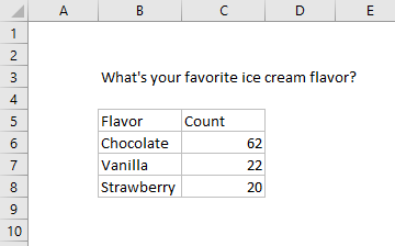
Note data does not include percentage breakdown — this is handled directly in the chart.
How to make this chart
- Select the data, then Insert > Pie chart on the ribbon:
- Chose the first 2D pie option:
- Initial chart after insert:
- Select and delete the legend
- Add data labels:
- Select data labels, and set display to show category name and percentage with a new line separator:
- Set data label text to white (if desired)
- Final chart with title:
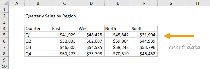
This chart shows quarterly sales data, broken down by quarter into four regions plotted with clustered columns.Clustered column charts work best when the number of data series and categories is limited. In order to make the data labels fit into a narrow space, the chart uses a custom number format ([>=1000]#,##0,“K”;0) to show values in thousands.
The data used to plot this chart is shown below:
How to make this chart
- Select the data and insert a column chart:
- Select the clustered column option
- Initial chart:
- Switch rows and columns to group data by quarter:
- After switching rows and columns:
- Move legend to top:
- Add data labels:
- Select data labels (one series at a time), and apply the custom number format for thousands:
- Set series overlap and gap width:
- Select and delete primary axis
- Select and delete gridlines
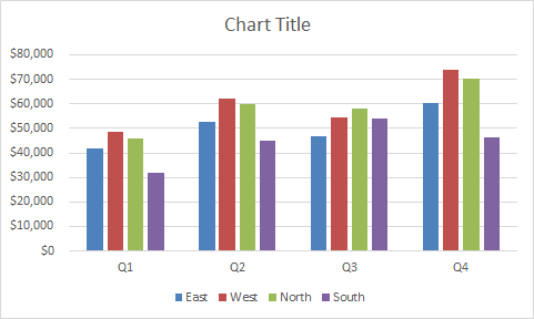
- Final stacked column chart:
At this point, you can finalize the chart by setting a title, and adjusting overall chart size, font size, and colors.
