Explanation
The goal is to calculate a tax of 6% on amounts up to 20,000 and a tax of 10% on amounts of 20,000 or greater. This problem illustrates how to use the IF function to return different calculations. At the core, this formula uses a single IF function . The logical test is based on this expression:
B5<=limit
When B5 (the current amount) is less than the limit in cell F6 (20,000), the test returns TRUE and the IF function applies rate1 only:
B5*rate1
When B5 is greater than 20,000, the test returns FALSE and the IF function applies rate1 and rate2 :
limit*rate1+(B5-limit)*rate2
Translation:
- Calculate rate1 by multiplying the limit (20,000) by 6% (F4).
- Calculate rate2 by subtracting the limit from the amount, and multiplying the result by 10% (F5)
- Add #1 and #2 together
Without named ranges
Named ranges can make formulas easier to write and read. The same formula without named ranges looks like this:
=IF(B5<=$F$6,B5*$F$4,$F$6*$F$4+(B5-$F$6)*$F$5)
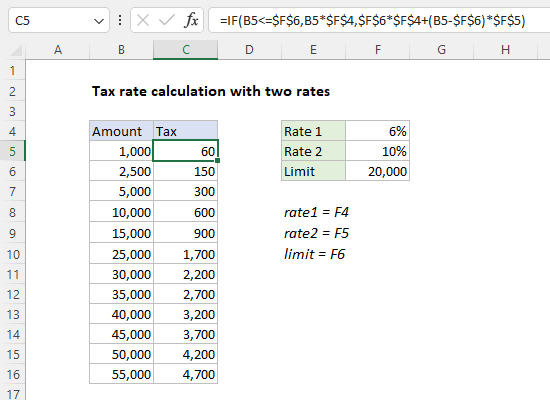
References to F4, F5, and F5 are locked to prevent changes when the formula is copied down the table. Notice B5 is still a relative reference because we want the reference to change as the formula is copied.
Explanation
In geometry, the area enclosed by a circle with radius (r) is defined by the following formula: πr 2
The Greek letter π (“pi”) represents the ratio of the circumference of a circle to its diameter. In Excel, π is represented in a formula with the PI function , which returns the number 3.14159265358979, accurate to 15 digits:
=PI() // returns 3.14159265358979
To square a number in Excel, you can use the exponentiation operator (^):
=A1^2
Or, you can use the POWER function :
=POWER(A1,2)
Rewriting the formula =πr2 as an Excel formula to for the example, we get:
=PI()*B5^2
Or:
=PI()*POWER(B5,2)
The result is the same for both formulas. Following Excel’s order of operations , exponentiation will occur before multiplication.
