Quick Links
- Quick Start
- Examples
- Troubleshooting
- Training
If you’ve ever applied conditional formatting with your own formula, you know the hardest part is making sure the formula actually works.
The problem is that the formula area in a conditional formatting rule isn’t very friendly. You don’t get highlighted cell references, you don’t get function autocomplete…heck….you don’t even get screen tips.
As a result, it’s hard to “see” if a formula is going to work until after you save the rule. If it doesn’t, you have to use trial and error:
- Edit the rule
- Edit the formula using your “best guess”
- Save the rule to see what happens
- Repeat as needed
This isn’t much fun, and it can be really frustrating when you run into a tricky problem.
Luckily, there’s an easy fix: dummy formulas.
A better way - test with dummy formulas
With more complicated conditional formatting formulas, the key is to test the rule with “dummy” formulas first, before you create the rule. This may at first seem impossible — how can you test a conditional formatting formula without applying a conditional format?
The trick is understanding that you can think of conditional formatting as an “overlay” of invisible formulas that sit on top of the cells. When a formula in the overlay returns TRUE for a given cell, the formatting is applied.
So, to test a conditional formatting rule, you just need to build a set of “dummy” formulas on the worksheet that simulates the overlay.
I like to put the test formulas over to the side of the data, lined up with the rows. This makes it easy to set up and match references.
Then, simply write the first formula by referencing the upper left cell in the data. This will be the active cell when the conditional formatting rule is created.
Video: Test conditional formatting with dummy formulas
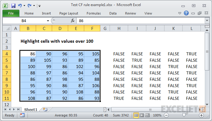
Example 1 - Simple Formula
For example, say you have numbers in a table, and you want to highlight values over 100.
Note: Excel contains a conditional formatting “preset” that will highlight values “greater than”, so it’s not necessary to use a formula to do this. We are just using a basic formula as an example.
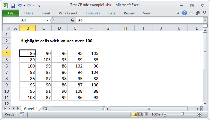
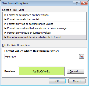
We have plenty of space to the right, so we’ll add our dummy formulas there. In cell H4, add the first formula. In this case, we want to use:
=B4>100
Why B4? Because B4 corresponds to the active cell we’ll have when we define the actual conditional formatting rule.
Now copy the formula across and down. You only need to copy down as many rows as you want to test. In this case, with a small set of data, we can easily test all rows.

Notice we get a TRUE or FALSE value in every cell. If we check a few references, you can see that each formula is evaluating a cell in the data, relative to B4. All references to B4 have changed, since B4 was entered as a relative address.
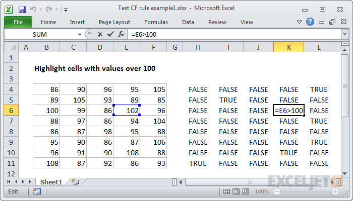
Checking references - each formula refers to a cell relative to B4
Now simply imagine these results transposed directly on top of the data. Wherever you see a TRUE value, the conditional formatting will be applied:
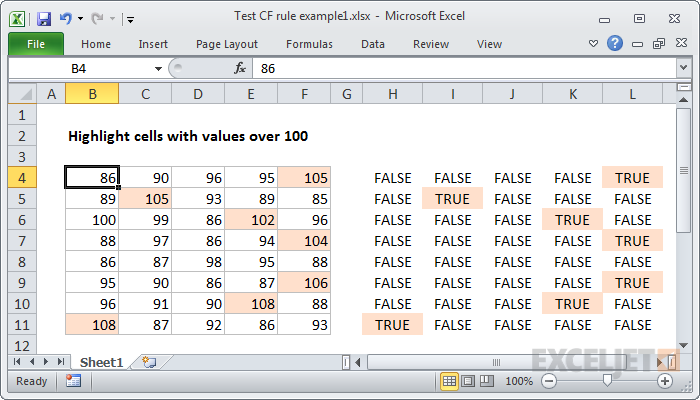
Notice that TRUE values are correctly marking the values > 100 in the data (manually highlighted)
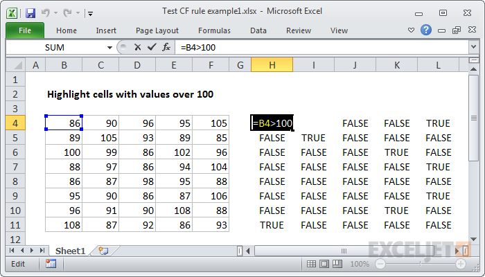
The dummy formula looks good, so let’s try it out in a conditional formatting rule.
First, copy the formula in the upper left cell of the dummy formulas – that’s H4 in this case.
Next, select the data and define a new conditional formatting rule.
Data selected - note the active cell is B4
Paste the formula into the box, and set the format.
Ready to save the new rule
Success! All cells with values over 100 highlighted:
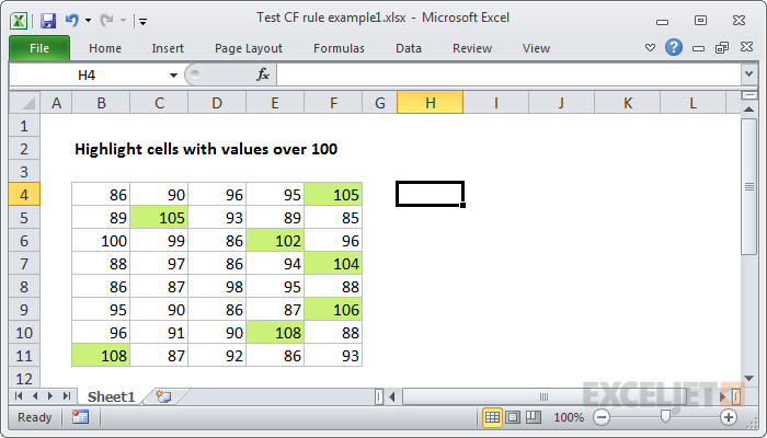
Final conditional formatting applied with a formula, with dummy formulas removed.
Example 2 - a more complicated formula
That was a simple example, so let’s try the same approach with a more complicated formula.
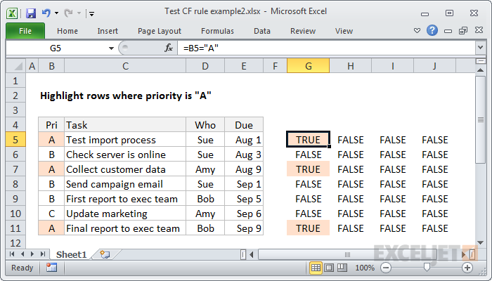
Let’s create a rule that highlights rows in a table based on the value in one column. In this case, we’ll highlight tasks with a priority of “A”.
<img loading=“lazy” src=“https://exceljet.net/sites/default/files/styles/original_with_watermark/public/images/articles/inline/CF_example2_start.png?itok=QqFucNzj" onerror=“this.onerror=null;this.src=‘https://blogger.googleusercontent.com/img/a/AVvXsEhe7F7TRXHtjiKvHb5vS7DmnxvpHiDyoYyYvm1nHB3Qp2_w3BnM6A2eq4v7FYxCC9bfZt3a9vIMtAYEKUiaDQbHMg-ViyGmRIj39MLp0bGFfgfYw1Dc9q_H-T0wiTm3l0Uq42dETrN9eC8aGJ9_IORZsxST1AcLR7np1koOfcc7tnHa4S8Mwz_xD9d0=s16000';" alt=“Problem - highlight tasks with a priority of “A” - 9”>
Need to highlight all rows with a priority of “A”
This is a classic problem in conditional formatting. The formula will require a mixed reference, but mixed references can be hard to understand when you aren’t able to see references on the worksheet. However, by using dummy formulas, we can easily test and perfect a rule.
As before, the first step is to figure out where to put the test formulas. We have plenty of room to the right, so we’ll start in cell G5.
Since we want to highlight tasks with a priority of “A”, we’ll use this formula to start:
=B5="A"
After I copy the formulas across and down, this is what we have:
Not going to work - only values in column B will be highlighted (orange shading manually applied)
Notice that we are getting a result of TRUE where the priority is “A”, but only for values in column B. It’s a good start, but it will only highlight cells in the first column.
We need to adjust the formula so that it returns TRUE for the entire row. To do this, we need to use a mixed reference in the formula to lock the column. The revised formula is:
=$B5="A"
When I copy this new formula across our test range, we get what we need:
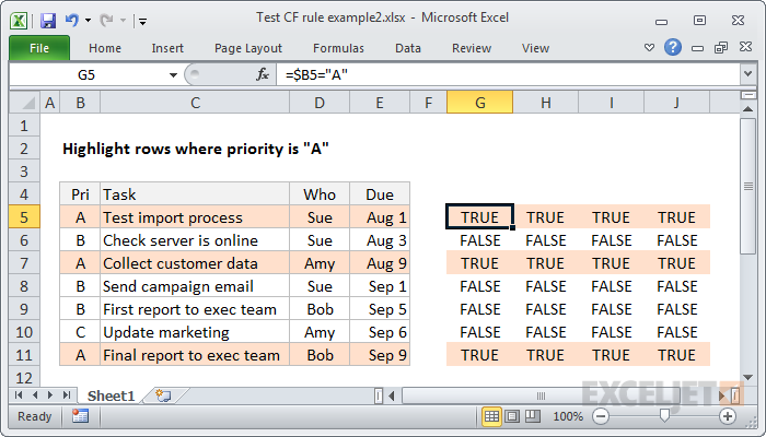
With the column locked, we get an entire row of TRUE’s when the priority is “A” (orange shading manually applied)
See how the dummy formulas will work? Imagine them as an overlay on the data itself.
Now let’s created the conditional formatting rule. First, select the data:
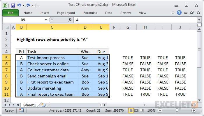
Data selected, and ready to create new rule (note active cell is B5)
Finally, let’s create the rule, using the formula in the upper left:
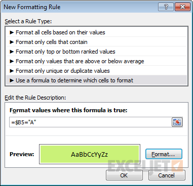
Formula pasted from G5
As you can see, the new rule works perfectly the first time.
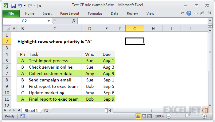
Conditional formatting working as expected (dummy formulas removed)
Conclusion
The next time you need to apply conditional formatting with a more complicated formula, set up dummy formulas next to the data, and fine tune the formula until you get TRUE values where you need them. By working directly on the worksheet, you have full access to all of Excel’s formula tools, and you can easily troubleshoot and adjust the formula until it works perfectly.
See more conditional formatting formulas here
A few days ago, I posted this conditional formatting puzzle :
Given a date, what formula will highlight other dates in the same month and year?

Here’s the list:
Option #1 - Extract with MONTH and YEAR and test with AND Option #2 - force dates to first of month and compare Option #3 - force dates to last of month and compare Option #4 - concatenate year and month and compare Option #5 - concatenate year and month with TEXT and compare
Download the practice worksheet attached below and try them out yourself. In the worksheet, cell E2 is named “date”.
If you need a quick recap on how to use a formula with conditional formatting, see: How to apply conditional formatting with a formula . Here is another article on Conditional formatting based on a different cell.
The purpose of these formulas is to automatically highlight dates in the table whenever the date in E2 changes.
Option #1- Extract with MONTH and YEAR and test with AND
The “obvious” solution (if you’re an Excel nerd :)) is one that uses the AND function along with MONTH and YEAR. It looks like this:
=AND(YEAR(B4)=YEAR(date),MONTH(B4)=MONTH(date))
This formula uses the AND function to test two conditions:
YEAR(B4)=YEAR(date) // is the year the same?
MONTH(B4)=MONTH(date) // is the month the same?
Both of these conditions use the equal sign to force a TRUE or FALSE result. If both return TRUE, AND returns TRUE and the conditional formatting is triggered.
Pros - intuitive, straightforward Cons - requires five function calls and four references
I also like this formula because it builds on simple functions that you absolutely need to know: MONTH, YEAR & AND.
Option #2- force dates to first of month and compare
Another interesting solution is to pull out the month and year from each date and use these values to build “first of the month” dates, which are then compared. The formula looks like this:
=DATE(YEAR(B4),MONTH(B4),1)=DATE(YEAR(date),MONTH(date),1)
There are two main parts of the formula. On the left of the equal sign, the formula extracts the year and month values from B4, then uses those values to create a new date with the day value hard-coded as 1. On the right, the same thing happens with the date in date ($E$2).
=DATE(YEAR(B4),MONTH(B4),1)=DATE(YEAR(date),MONTH(date),1)
=DATE(2015,2,1)=DATE(2015,6,1)
=42036=42156*
=FALSE
- 42036 is the date serial number for 1-Feb-2015 and 42156 is the serial number for 1-Jun-2015, which is how Excel evaluates the dates internally.
In each case, the year and month values are extracted, and used to create a new date where the day value is hard-coded as 1. Effectively, this ignores day completely by making it the same for each date.
Finally, the two dates are tested for equality.
Pros - fairly intuitive Cons - requires six function calls and four references
What I like about this formula is the creative thinking — the “trick” of forcing the day to 1. You’ll find these kind of tricks are everywhere in more complex Excel formulas.
Option #3 - force dates to last of month and compare
Similar to option #3, another clever idea from reader Eric Kalin is to force dates to “last of month” and compare. This is a nice solution because Excel has a dedicated function for getting the last day a month: EOMONTH. The formula looks like this:
=EOMONTH(B4,0)=EOMONTH(date,0)
This formula can be summarized like this: get the last of month using the date in B4 and compare it to the last day of month based on the date in $E$2.
Pros - compact and economical; just two function calls and two references Cons - need to know and understand EOMONTH
Overall, a very nice formula that stands out for its simplicity.
Option #4 - concatenate year and month and compare
Yet another approach is to extract and concatenate the year and month values for each date, then compare the result:
=MONTH(B4)&YEAR(B4)=MONTH(date)&YEAR(date)
This may not be a solution you’d think of initially, because the idea of concatenating numbers is a little weird.
If you concatenate, say, 11 (November) with the year 2015, you’ll get “112015”, which is likely not a value you’d recognize at first glance. However, to Excel, it’s just a string (text value), and Excel will be happy to compare it with any other string for you. So, here’s what the formula looks like for cell B4 and cell $E$2 as it’s solved:
=MONTH(B4)&YEAR(B4)=MONTH(date)&YEAR(date)
="22015"="62015"
=FALSE
Pros - logical and relatively compact (4 function calls) Cons - need to know about concatenation
Option #5 - concatenate year and month with TEXT and compare
Finally, here is another formula that relies on the idea of concatenating the month and year together. However, this formula uses the TEXT function and a custom number format, rather than concatenating manually with the ampersand (&) operator:
=TEXT(B4,"myyyy")=TEXT(date,"myyyy")
TEXT is a useful function that allows you to convert a number to text in the text format of your choice. In this case the format is the custom date format “myyyy”, which translates to: month number without leading zeros & 4-digit year.
Like #4 above, the result is the same as concatenating the month and year manually. Solving with B4 and date ($E$2):
=TEXT(B4,"myyyy")=TEXT(date,"myyyy")
="22015"="62015"
=FALSE
Pros - simple and compact (2 function calls) Cons - need to understand TEXT
What’s the best option?
Well, in many cases, the best option is the one you know :)
If you spend a lot of time with Excel formulas, you’ll notice an obsession (in yourself, and in others) with compact and elegant formulas. It’s hard not to be delighted by a clever and efficient formula. And it’s true that shorter formulas offer less chance of making a mistake, since you aren’t wrangling as many parentheses and references.
But all that said, Excel is a vehicle, not a destination. Unless you build models professionally, or analyze huge data sets (where efficiency really counts), your boss probably doesn’t care what formula you use as long as it gets the job done accurately, and is straightforward to understand.
Are you looking for more conditional formatting formulas ?
