Explanation
In this example, we have comma-separated text in column B. The goal is to split the text in column B into columns D through G while at the same time converting the numbers to true numeric values. The challenge is that TEXTSPLIT always returns text, so we need a way to convert the numbers while leaving the text values alone.
The problem with TEXTSPLIT
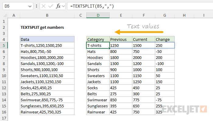
To split the text in column B into separate columns, we can use the TEXTSPLIT function with a simple formula like this:
TEXTSPLIT(B5,",")
This seems to work great. But the problem is that the numbers in columns E, F, and G aren’t really numeric values . Instead, they are text values, as you can see by the way Excel aligns them to the left:
If you use a function like SUM to sum these numbers up, the result will be zero . How can convert these numbers as text to actual numeric values? Well, one option is to use the VALUE function.
Adding the VALUE function
The VALUE function is designed to convert text that appears in a recognized format (i.e. a number, date, or time format) into a numeric value. If we wrap the VALUE function around the TEXTSPLIT function, this is the result:

Notice the numbers in columns E, F, and G are now actually numeric values, as we can see by the way Excel right-aligns them. However, we now have a new problem — the VALUE function has corrupted the text values in column D. This happens because when VALUE tries to convert the text to a number, the operation fails with a #VALUE! error. What we need is a way to selectively convert the “numbers as text” to numbers while leaving the text values alone. We can do that with the IFERROR function.
Adding the IFERROR function
The IFERROR function returns a custom result when a formula generates an error, and a standard result when no error is detected. The syntax for IFERROR looks like this:
=IFERROR(value,value_if_error)
To illustrate how this works, we can start by adding IFERROR like this:
=IFERROR(VALUE(TEXTSPLIT(B5,",")),"x")
Notice we have simply embedded the original formula above into IFERROR as the value argument, then provided the value “x” for value_if_error. The result looks like this:
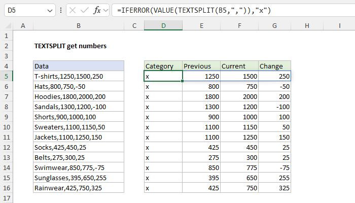
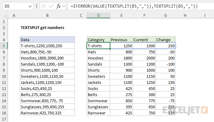
The “x” in column D tells us that IFERROR has encountered an error in this column, which is created when VALUE tries to convert the text values into numbers. The final step is to replace the “x” with the original text value. We can do that by simply repeating the original TEXTSPLIT formula. The final formula looks like this:
=IFERROR(VALUE(TEXTSPLIT(B5,",")),TEXTSPLIT(B5,","))
The result in the worksheet looks like this:
Optimizing with the LET function
The formula above works fine, but it would be inefficient with a large amount of data because we are running the same TEXTSPLIT operation twice. One way to improve performance is to use the LET function like this:
=LET(array,TEXTSPLIT(B5,","),IFERROR(VALUE(array),array))
In this formula, the result from TEXTSPLIT is assigned to a variable named “array”. We then use array inside the IFERROR and VALUE functions as above. The key difference is that TEXTSPLIT runs just one time .
Explanation
This example shows a workbook designed to apply discounts based on seven pricing tiers. The total quantity of items is entered as a variable in cell C4. The discount is applied via the unit costs in E7:E13, which decrease as the quantity increases. The first 200 items have an undiscounted price of $1.00. The next 300 items have a discounted unit price of $0.90. The next 250 items have a unit price of $0.80, and so on.
The main challenge in this problem is calculating the correct quantities in the range D7:D13. The goal is to write a formula to distribute the quantity in C4 (850) into separate tiers based on the thresholds entered in C7:C13. Once these numbers are in place, calculating the line totals in column F is a simple matter of multiplying the quantity in column D by the unit cost in column E.
Understanding the problem
As mentioned above, the challenge in this example is figuring out a good way to calculate quantities per tier in the range D7:D13. Essentially, we need to distribute the quantity in cell C4 into separate “buckets” according to the thresholds given in C7:C13. We fill one bucket at a time, beginning with the first tier. Once that bucket is full, we move on to the next bucket. We continue in this way, filling up each bucket in turn until we have exhausted the quantity in cell C4. Translating this idea into cells on the worksheet, the logic we need to implement looks like this:
- If the quantity is less than or equal to the previous threshold, we are done and the result should be 0. In other words, the current tier has not been reached.
- If the quantity exceeds the current threshold, the result is the difference between the current and previous threshold. We subtract the previous threshold from the current threshold.
- Otherwise, the result is the difference between the quantity and the previous threshold. We subtract the previous threshold from the quantity.
Below, I explain two ways to solve this problem. The first method keeps the worksheet structure intact and uses the MAP function to generate all tier quantities simultaneously. This method requires Excel 365. The second method restructures the worksheet and uses a more straightforward traditional formula that will work in all versions of Excel.
MAP solution in Excel 365
The worksheet shown above uses a single formula in cell D7 to calculate all quantities in D7:D13:
=LET(
  quantity,C4,
  thresholds,C7:C13,
  prevthresholds,DROP(VSTACK(0,thresholds),-1),
  MAP(thresholds,prevthresholds,LAMBDA(a,b,
    IF(quantity<=b,0,
      IF(quantity>a,a-b,quantity-b))
  ))
)
At a high level, we use the MAP function to calculate the final result. MAP is designed to work with like-sized arrays, iterating through an array one element at a time and performing a custom calculation at each step. The formula works like this:
First, we define the variable “quantity” as equal to cell C4 and the variable “thresholds” as equal to the range C7:C13:
quantity,C4,
thresholds,C7:C13,
This step makes the formula easier to read and more portable since the only worksheet references occur in the first two lines. Next, we need to create an array of “previous thresholds” in order to implement the logic explained above. To do that, we define “prevthresholds” with the VSTACK function and the DROP function like this:
prevthresholds,DROP(VSTACK(0,thresholds),-1)
Working from the inside out, we first use VSTACK to insert a zero at the start of the “thresholds” array. This effectively “pushes down” the items in the array so that the current and previous thresholds are “aligned”, which allows MAP to work with both values at the same time. Then, we use the DROP function to remove the final last value since we don’t need it. After this code runs, we have an array that contains seven numbers:
{0;200;500;750;1500;3000;5000}
Note this array is similar to the original threshold values, except we have a zero as the start and the last value has been removed. Next, we use the MAP function to generate the quantities per tier like this:
  MAP(thresholds,prevthresholds,LAMBDA(a,b,
    IF(quantity<=b,0,
      IF(quantity>a,a-b,quantity-b))
  ))
Notice the first two arguments are the arrays created in the previous steps. Next, we have a custom LAMBDA calculation . Inside the LAMBDA, “a” is the “thresholds” array, and “b” is the “prevthresholds” array. (See our MAP page for an explanation of this structure). The logic is implemented with a nested IF formula:
LAMBDA(a,b,
    IF(quantity<=b,0,
      IF(quantity>a,a-b,quantity-b))
- If the quantity is less than or equal to the previous threshold, the result should be 0.
- Otherwise, if the quantity exceeds the current threshold, subtract the previous threshold from the current threshold.
- Otherwise, subtract the previous threshold from the quantity.
MAP iterates through each of the seven thresholds and generates a result for each tier using the logic above. The final result is an array of seven quantities, one for each tier:
{200;300;250;100;0;0;0}
The array lands in cell D7, and the values spill into the range D7:D13.
Note: This problem is a good example of how new functions in Excel can be used to solve hard problems neatly. However, it is also a case where choosing MAP is not obvious. The trick here is to create an array of “previous thresholds” so that current and previous values are simultaneously available. Knowing when and how to do this is part of the learning curve of new functions like MAP. I’m sure there are many ways to solve this problem with other dynamic array functions.
MIN and MAX alternative
The logic inside the nested IF in the formula above can be “compressed” by replacing IF with the MIN and MAX functions like this:
=LET(
quantity,C4,
thresholds,C7:C13,
prevthresholds,DROP(VSTACK(0,thresholds),-1),
MAP(thresholds,prevthresholds,LAMBDA(a,b,MAX(0,MIN(quantity,a)-b)))
)
Both formulas return the same results, but the second formula is more concise. The trade-off is that it is more difficult to understand at a glance, especially for those new to this technique.
Traditional solution for older versions of Excel
In older versions of Excel that do not support dynamic array formulas, I recommend changing the worksheet’s structure to make it easier to solve with a more traditional formula by inserting “previous threshold” values before the existing threshold values. You can see this approach in the worksheet below:
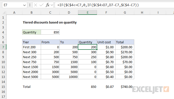
In this worksheet, the “From” column contains previous threshold values, and the To column contains the original threshold values. The formula in cell E7, copied down, looks like this:
=IF($C$4<=C7,0,IF($C$4>D7,D7-C7,$C$4-C7))
As the formula is copied down, it calculates the quantity for each tier, following the same logic as the MAP formula but without the dynamic array capabilities. This approach processes each row individually.
- If the quantity is less than or equal to the previous threshold, the result should be 0.
- Otherwise, if the quantity exceeds the current threshold, subtract the previous threshold from the current threshold.
- Otherwise, subtract the previous threshold from the quantity.
Like the MAP formula above, we can replace the nested IF structure with a more compact formula using MAX and MIN like this:
=MAX(0,MIN($C$4,D7)-C7)
Both formulas will return the same results.
Note: I created this example to show how Excel’s new MAP function can be used to solve tricky problems in an elegant way. Excel’s new functions are very powerful, but it’s often not clear how you would use a function like MAP. By the time I finished with the traditional formula approach, I was reminded yet again of the power of restructuring a worksheet to simplify a problem. Do not overlook this “one simple trick” to make hard problems easier to solve :)
