The Eomonth Function

The EOMONTH function is one of those little gems in Excel that can save you a lot of trouble. It’s a simple function that does just one thing: given a date, it returns the last day of a month.

This may seem a little silly — how hard can it be to figure out the last day of a month? — but it’s actually a bit tricky, since each month has a different numbers of days, and February changes in leap years.

Enter the EOMONTH function

EOMONTH takes two arguments: a start date, and months. Months represents the number of months to move in the future or past. So, for example, with May 12, 2017 in cell B5:

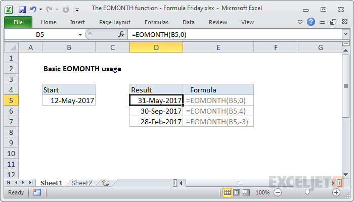
=EOMONTH(B5,0) returns May 31, 2017
=EOMONTH(B5,4) returns Sep 30, 2017
=EOMONTH(B5,-3) returns Feb 28, 2017

You can easily use EOMONTH to move through years as well:

=EOMONTH(B5,12) returns May 31, 2018
=EOMONTH(B5,36) returns May 31, 2020
=EOMONTH(B5,-24) returns May 31, 2015

You can also use EOMONTH to easily get the first day of the next month:

=EOMONTH(B5,0)+1 returns Jun 1, 2017

Notes on using EOMONTH

1. Make sure you give EOMONTH a proper date to start. You can use the DATE function if you need to assemble a date from scratch.
2. Make sure you apply date formatting to the result of EOMONTH, otherwise you may see just a big number.
3. If you want to move to the same date in past or future months, use the EDATE function .

Example formulas built on EOMONTH

Building on EOMONTH’s simple utility, you can build all kinds of useful formulas. Here are a few examples to give you some inspiration:

• Sum by month
• Days in month
• Get last working day in month
• Calculate retirement date
• Get first day of previous month

More formulas

We have more than 500 formulas examples , and high-quality video training if you like learning with a structured program.

I’ve been playing around with the TEXTJOIN and CONCAT functions this week. These are both new functions in Excel 2016, introduced in the Office 365 subscription service.

Both of these functions let you join (concatenate) text in different cells together. TEXTJOIN lets you join values with a delimiter of your choice, and has an option to ignore empty values. CONCAT simply mashes all values together without options.

What’s nice about both of these functions is that they can handle cell ranges.

That means you can do things like this:

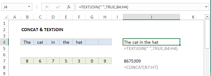
=TEXTJOIN(" ",TRUE,B4:H4) // J4
=CONCAT(B7:H7) // J7

Maybe you’re old enough to recognize that number ? :)

The ability to handle ranges is cool, because it makes it trivial to concatenate a large collection of cells with a simple formula - something that required annoying workarounds previously.

But I’m also intrigued about how this might be useful inside other formulas. In most programming languages, its common to split values into arrays, and join values back together again, after some kind of processing. For example, VBA has SPLIT and JOIN, and PHP has EXPLODE and IMPLODE, etc.

Inside an Excel formula, it’s not too hard to split values into an array:

=MID("apple",{1,2,3,4,5},1) // returns {"a","p","p","l","e"}

But once you have {“a”,“p”,“p”,“l”,“e”}, how you can you put it back together again?

Turns out, CONCAT and TEXTJOIN will let you do it, which solves a problem that’s bugged me for a long time:

=CONCAT({"a","p","p","l","e"}) // returns "apple"
=TEXTJOIN("",TRUE,{"a","p","p","l","e"}) // returns "apple"

Why does it matter?

To be honest, I’m not entirely how useful this is, since I’ve just started fiddling around with these functions. However, I think this might open the door to some interesting formulas that process values by looping through looping arrays. Here are a few ideas you might find interesting:

1. Uppercase text

=TEXTJOIN("",TRUE,(CHAR(CODE(MID(A1,{1,2,3,4,5},1))-32)))

The example above will uppercase “apple” > “APPLE” in A1. It’s a silly example, since you can do the same thing more easily with the UPPER function. But I think it shows nicely how you can loop through each character, make changes, then bring it all back together again with TEXTJOIN.

2. Strip non-numeric characters

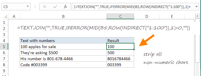
{=TEXTJOIN("",TRUE,IFERROR(MID(A1,ROW(INDIRECT("1:100")),1)+0,""))}

Note: this is an array function - use control + shift + enter.

This example will strip all non-numeric characters in A1. So, for example, you can take a phone number like “(801)-654-4466” and turn it into “8016544466”, which can then be formatted using a custom number format. You can do this same thing with the SUBSTITUTE function, but it’s more work. If you’re curious, here is a detailed explanation of how this formula works.

More examples of TEXTJOIN formulas .