Explanation
In the example shown, the goal is to enter a valid time based on days, hours, and minutes, then display the result as total hours.
The key is to understand that time in Excel is just a number. 1 day = 24 hours , and 1 hour = 0.0412 (1/24). That means 12 hours = 0.5, 6 hours = 0.25, and so on. Because time is just a number, you can add time to days and display the result using a custom number format, or with your own formula, as explained below.
In the example shown, the formula in cell F5 is:
=B5+TIME(C5,D5,0)
On the right side of the formula, the TIME function is used to assemble a valid time from its component parts (hours, minutes, seconds). Hours come from column C, minutes from column D, and seconds are hardcoded as zero. TIME returns 0.5, since 12 hours equals one half day:
TIME(12,0,0) // returns 0.5
With the number 1 in C5, we can simplify the formula to:
=1+0.5
which returns 1.5 as a final result. To display this result as total hours, a custom number format is used:
[h]:mm
The square brackets tell Excel to display hours over 24, since by default Excel will reset to zero at each 24 hour interval (like a clock). The result is a time like “36:00”, since 1.5 is a day and a half, or 36 hours.
The formula in G5 simply points back to F5:
=F5
The custom number format used to display a result like “1d 12h 0m” is:
d"d" h"h" m"m"
More than 31 days
Using “d” to display days in a custom number format works fine up to 31 days. However, after 31 days, Excel will reset days to zero. This does not affect hours, which will continue to display properly with the number format [h].
Unfortunately, a custom number format like [d] is not supported. However, in this example, since days, hours, and minutes are already broken out separately, you can write your own formula to display days, minutes, and hours like this:
=B5&"d "&C5&"h "&D5&"m"
This is an example of concatenation . We are simply embedding all three numeric values into single text string , joined together with the ampersand (&) operator .
If you want to display an existing time value as a text string, you can use a formula like this:
=INT(A1)&" days "&TEXT(A1,"h"" hrs ""m"" mins """)
where A1 contains time. The INT function simply returns the integer portion of the number (days). The TEXT function is used to format hours and minutes.
Explanation
In the worksheet shown, we have race results for an 800m race. The goal is to display time in minutes, seconds, and hundredths of a second (centiseconds). Dealing with times that include fractional seconds can be tricky in Excel. The default time format will only show whole seconds and it is not obvious how to display seconds in smaller units. The first step is to apply a custom number format that specifically includes placeholders for tenths, hundredths, or thousandths of a second as needed. However, several quirks in Excel make working with fractional seconds more difficult than you would expect. This article explains these quirks and provides tips and formulas to make the process easier.
Time values in Excel are fractions of 1, as explained on this page .
Number formats for time with seconds
The first step in working with seconds in smaller increments is to apply a suitable number format. The following custom number formats will display tenths, hundredths, or thousandths of a second as noted:
mm:ss.0 // tenths of a second (deciseconds)
mm:ss.00 // hundredths of a second (centiseconds)
mm:ss.000 // thousandths of a second (milliseconds)
If the time also includes hours, add a placeholder for hours like this:
[h]:mm:ss.0 // tenths of a second (deciseconds)
[h]:mm:ss.00 // hundredths of a second (centiseconds)
[h]:mm:ss.000 // thousandths of a second (milliseconds)
The square bracket syntax “[h]” tells Excel to treat the time as a duration that may exceed 24 hours. Without the brackets, times with durations greater than 24 hours will appear to reset to zero every 24 hours. Note when you add a placeholder for hours, you must enter time starting with hours. For example, enter “1:05:31.25” for “1 hour, 5 minutes, and 31.25 seconds” and “0:07:45.10” for “0 hours, 7 minutes and 45.10 seconds”. In short, you must enter time according to specified placeholders.
Excel’s number formats are a deep topic. See Excel Custom Number Formats for more information.
How to apply a custom time format
To enter and display time that includes a decimal value for seconds in Excel, you must first apply a custom format. The fastest way to do this is to use the Format Cells dialog box like this:
- Select the range of cells that will contain time values.
- Open Format cells with the keyboard shortcut Control + 1
- Go to the “Number” tab, then select “Custom.”
- In the “Type” field, enter mm:ss.00 for minutes, seconds, and hundredths of a second.
- Click the OK button to apply the format.

After the custom format is applied, you must enter the time in the format specified. For example, enter “01:45.73” for “1 minute, 45.73 seconds”.
Editing time in Excel
One of the frustrations of using a custom time format in Excel is that the format is not honored when editing an existing value. For example, you may have a time value like “01:50.82” in a cell but when you edit the cell, Excel will stubbornly present the time as “12:01:51 AM”, ignoring the custom time format:
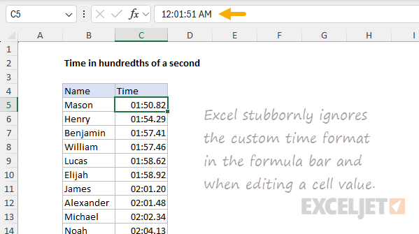
While you can still see and edit whole minutes and seconds, fractional seconds are no longer visible. Often, it is easiest to enter the complete time again. In cases where you need to edit time more easily, one option is to set up a helper column that contains the time as a text value, then convert the text to a proper time with the TIMEVALUE function as seen below:
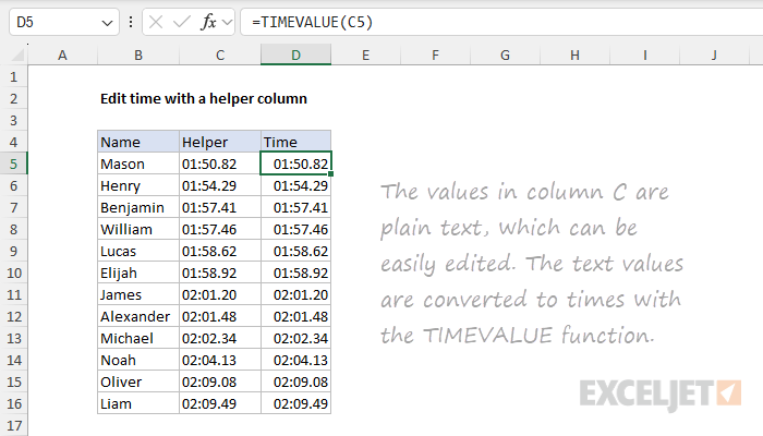
The advantage of this approach is the text in column C is easy to edit without re-entering the time. If you are entering the times by hand, one frustration is that Excel really likes to convert text into numbers , which defeats the idea of entering text. If you have trouble entering times as text, prepend the text with a single quote (’) like this:
'01:50.82 // time as text value
The single quote will force Excel to treat the value as text, and the single quote will not display on the worksheet.
Extracting fractional seconds from a time
When you have times in Excel that contain hundredths of a second, how can you extract seconds including any fractional part? This is a puzzling problem. Although Excel offers the SECOND function to extract seconds from a time, SECOND will round fractional seconds to the nearest whole number . For example, with the worksheet above, if we feed Mason’s time in C5 and Henry’s time in C6 into the SECOND function, we get back 51 and 54:
=SECOND(C5) // returns 51.0
=SECOND(C6) // returns 54.0
That means we can’t use SECOND to extract seconds that contain a decimal value without losing precision. The solution is to use a manual formula to extract seconds like this:
=MOD(C5*1440,1)*60
This formula works to extract fractional seconds from a time in three steps. The first step is to multiply by 1440. Excel stores dates and times as serial numbers where one day is 1.0. Since there are 1440 minutes in a day (24 hours x 60 minutes), multiplying the time by 1440 converts the time into minutes as a decimal value. With the time in C5 of 01:50.82 (stored as the decimal value 0.001282639 by Excel), we get 1.847:
=MOD(1.847,1)*60
The next step is to use the MOD function to get fractional seconds. MOD is a shortcut here. Since we already have decimal minutes from the previous step, providing 1 as the divisor is a simple way to remove the integer portion of the number (whole minutes) and return only the decimal part, 0.847:
=MOD(1.847,1)*60
=0.847*60
The third and final step is to multiply by 60 to convert decimal minutes to decimal seconds. Multiplying 0.847 x 60 results in 50.82 seconds:
=0.847*60
=50.82
This matches the value for seconds seen in cell C5. The worksheet below shows the result from all times in column C.
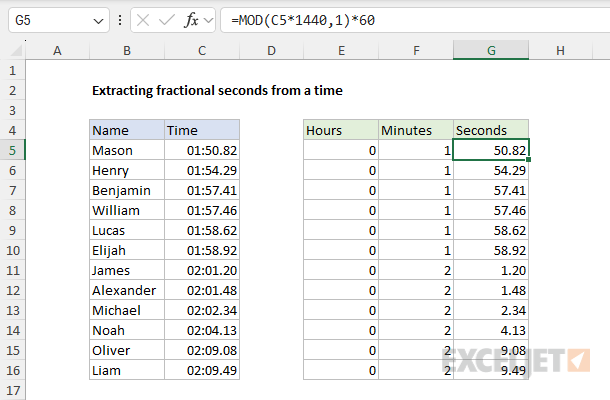
The formulas used to extract hours, minutes, and seconds are as follows:
=HOUR(C5) // extract hours
=MINUTE(C5) // extract minutes
=MOD(C5*1440,1)*60 // extract fractional seconds
All three results are formatted as numbers, not times.
A formula to create a time with fractional seconds
How do you create a time with fractional seconds with a formula? The first thing to know is that Excel’s TIME function doesn’t handle decimal values for hours, minutes, or seconds. You can see this behavior in the formulas below:
=TIME(3,0,0) // returns 3 hours
=TIME(3.5,0,0) // returns 3 hours
Although hours is 3 in the first formula and 3.5 in the second, both formulas return the same result. TIME simply removes the decimal part (0.5) during calculation. Likewise, if we try to provide 30.5 for seconds , the decimal portion is discarded. Both formulas below return exactly 30 seconds:
=TIME(0,0,30) // returns 30 seconds
=TIME(0,0,30.5) // returns 30 seconds
Consequently, to create a time that includes decimal values for hours, minutes, or seconds, we can’t use the TIME function. One solution is to use a purely math-based formula like this:
=(hours/24)+(minutes/1440)+(seconds/86400)
You can hardcode decimal values for hours, minutes, and seconds directly into this formula, or plug in values from cell references on a worksheet. You can see how this formula works in the worksheet below, where the formula in F5, copied down, is:
=(B5/24)+(C5/1440)+(D5/86400)
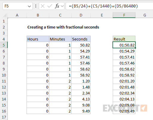
The final result is a list of original times above, complete with fractional seconds.
