Above: Tracking public COVID-19 testing data in Excel with Power Query
In this article, I want to share a quick example of how to track testing for COVID-19 using Excel and publicly available data. This is a bare bones tutorial, focused only on the basics of connecting Excel with publicly available data.
The end result is a simple Excel table that shows the most recent testing data by state. The data is fetched and “shaped” with Power Query , then dropped back into Excel, where it can be refreshed with a single click. The approach is general and can be used with all kinds of public data. The complete Excel file is attached below for reference.
The data
Requirements
This project depends on Power Query, so you’ll need Excel 2013 or later on Windows. On the Mac, you can refresh queries with Office 365 Excel, but I don’t think you can edit or create queries yet? I’ll update when I have better info.
Getting the data into Excel
The best tool for the job is Power Query. Power Query is part of Microsoft’s BI suite. In a nutshell, Power Query is a tool for fetching, cleaning, and shaping data.
If you are new to Power Query, be aware that it has a vast feature set and an intimidating interface. Even if you spend a lot of time in Excel, you are going to feel like you’ve landed in an alien world. Familiar, yet distinctly different.
Never fear, we are going to keep things as simple as possible. There are many ways this example can be improved or embellished once you get things working.
High-level overview
To orient you, here are the high level steps we are going to perform:
- Create new excel workbook
- Create a new query to fetch data
- Edit query to shape data
- Load data back to Excel Table
- Add formulas as desired
The first two steps happen in Excel. The last two steps are done in power query. Once you have the query set up, you can right-click inside the table and select refresh. Fresh data will be collected, and the data will be shaped according to the steps defined in the query.
Steps to create the query
April 2 - the data for this project has been changing as more columns are tracked in the same file. The steps below need to be updated slightly, but the query in the attached Excel workbook is current.
These are the steps I used to create the query that fetches data from the tracking website.
- Click Data > Get Data > From web
- Enter the url: https://covidtracking.com/api/states.csv and click OK
- Click the Transform Data button to launch Power Query:
- Power Query will automatically add three steps: Source, Promote Headers and Change type. If you select a step, you can see what it does.
- Remove the automatic “Change Type” step. Hover and click on the “X” on the left. We will manually change type again below to make the query more resilient.
- Control-click to select five columns: state, positive, death, dateModified, totalTestResults. Then, right-click on a select column and choose “Remove other columns”.
- For each column select the “ABC”, and Change Type: state (text), positive (whole number), death (whole number), dateModified (date time), totalTestResults (whole number).
- Drag to reorder columns: state, positive, death, dateModified, totalTestResults.
- Rename columns to: state, positive, death, modified, total. Double-click header to rename columns.
- Sort data by the “positive” column in descending order.
- Rename Query to “states”:
- Verify you have five columns of data like this:
- Click Close and Load button on Data tab of ribbon.
- The data will end up in an Excel Table called “states”
Refreshing data
To fetch the latest data, right-click in the table and select “Refresh”.
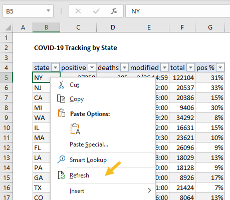
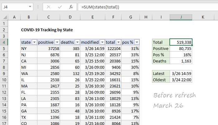
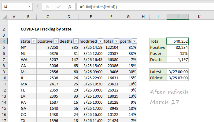
Power Query will pull down a fresh set of source data, run through the steps defined above, and deliver the result back to Excel. The screens below show the data on March 26 (before refresh, and March 27 (after refresh).
Back in Excel
Once the data is in an Excel table, I added a column called “pos %” that calculates what percentage of total tests are positive with this formula:
=[@positive]/[@total] // calculate percent positive
This is just something I was curious about. It could be added in Power Query instead (before loading to Excel) but to keep things simple, the formula was added manually in Excel. Since it lives in an Excel Table , it stays up to date when date changes.
Then I added formulas to summarize the data:
=SUM(states[total]) // J4
=SUM(states[positive]) // J5
=J5/J4 // J6
=SUM(states[deaths]) // J7
=MAX(states[modified]) // J9
=MIN(states[modified]) // J10
Note: most of these formulas use structured references , the formula syntax for Excel Tables.
How to edit the query
- Click Queries and Connections on the Data tab of the ribbon
- Double click the “states” query to edit
More data
Here are a few more Coronavirus datasets with sample files you can try out.
Notes
- Many of the articles I’ve read about COVID-19 warn against focusing on testing only, because it can distract from the more serious problem, exponential spread of a contagious disease. To be clear, this article’s only purpose is to show an example of how to get public data into Excel.
- I’ve posted more examples of Coronavirus datasets you can download in this article .
Dynamic Arrays are one of the biggest changes ever to Excel’s formula engine. With 6 brand new functions that directly leverage dynamic arrays, they solve hard problems in Excel that have vexed even power users for decades. However, Dynamic Arrays are only available in Office 365 , they are not available in Excel 2016 or 2019, and won’t work in any older version.
For those not using Office 365, this page provides some alternative formulas that work in older versions of Excel. It’s important to understand however, that none of the alternatives will spill multiple results onto the worksheet into a spill range like a native dynamic array formula. This behavior is limited to the Office 365 version of Excel.
Remember also that Pivot Tables can be used to solve many of these same challenges.
New dynamic functions
For reference, the 6 new dynamic array functions are listed in the table below. Click a function name for an overview and examples of usage.
| Function | Purpose |
|---|---|
| FILTER | Filter data and return matching records |
| RANDARRAY | Generate an array of random numbers |
| SEQUENCE | Generate an array of sequential numbers |
| SORT | Sort range by column |
| SORTBY | Sort range by another range or array |
| UNIQUE | Extract unique values from a list or range |
ALTERNATIVES
This section contains alternative formulas that perform some of the same tasks as the functions in the table above. In almost all cases, the formulas are more complex and clunky than an equivalent dynamic array formula. At the same time, these formulas should work in almost any version of Excel.
Note: several of these formulas are traditional array formulas and need to be entered with control + shift + enter. If you are working with them in Dynamic Excel, you don’t need to use control + shift + enter, Excel will handle the array operations automatically.
Sorting
Dynamic Excel provides two new functions to handle sorting with formulas: SORT and SORTBY . These functions make it easy to sort data by one or more columns, and even sort data by a custom list. However, if you are using an older version of Excel, you still have some options for sorting with a formula:
- Basic numeric sort formula
- Basic text sort formula
- Sort numbers ascending or descending
- Random sort formula
Filtering and extracting
Filtering and extracting data with formulas in Excel has always been a challenging problem. Dynamic Excel provides a special function, just for this purpose: the FILTER function . if you are using an older version of Excel, there are various ways to approach the problem.
- Extract all matches with helper column
- Extract all partial matches
- Extract multiple matches into separate columns
- Extract multiple matches into separate rows
Unique values
Dynamic Excel provides a dedicated function for working with unique values: the UNIQUE function . In other versions of Excel, you’ll need to cobble together solutions based on several other functions.
For counting unique values:
- Count unique numeric values in a range
- Count unique numeric values with criteria
- Count unique text values in a range
- Count unique text values with criteria
- Count unique values in a range with COUNTIF
For extracting unique values, and other tasks:
- Highlight unique values
- Data validation unique values only
- Extract unique items from a list
- Sort and extract unique values
Remember: Pivot Tables also provide good tools for listing and counting unique values.
Sequential values
One of the new Dynamic Array functions is SEQUENCE , specifically designed to generate numeric sequences. With controls for the start and step value, and the ability to output results in rows, columns, or both, SEQUENCE is a flexible tool for generating sequential dates, times, and all manner of numbers. If you are using an older version of Excel, there are other ways to create numeric sequences, but they are not as convenient. Commonly, you’ll see solutions that use the ROW function together with INDIRECT . Here are some examples:
- Sum bottom n values
- Sum top n values
- Count day of week between dates
- Strip non-numeric characters
Random values
The RANDARRAY function is also new in Dynamic Excel. RANDARRAY can generate random decimal or integer values in columns, rows, or two-dimensional arrays. The beauty of RANDARRAY is that you can ask for more than one random number at the same time. This is a huge benefit when building formulas that need to perform random sorts, or random item selection.
In older versions of Excel, you will typically use either the RAND function (decimal values) or the RANDBETWEEN function (integers) to perform the same tasks.
- Random sort formula
- Random date between two dates
- Random number from a fixed set of options
