Purpose
Return value
Syntax
=TRUNC(number,[num_digits])
- number - The number to truncate.
- num_digits - [optional] The precision of the truncation (default is 0).
Using the TRUNC function
The TRUNC function returns a truncated number based on an (optional) number of digits. For example, TRUNC(4.9) will return 4, and TRUNC(-3.5) will return -3. The TRUNC function does no rounding, it simply truncates as specified.
The TRUNC function takes two arguments : number and num_digits . Number is the numeric value to truncate. The num_digits argument is optional and specifies the place at which number should be truncated. Num_digits defaults to zero (0).
Examples
By default, TRUNC will return the integer portion of a number:
=TRUNC(4.9) // returns 4
=TRUNC(-3.5) // returns -3
To control the place at which number is truncated, provide a value for num_digits .
=TRUNC(3.141593) // returns 3
=TRUNC(3.141593,0) // returns 3
=TRUNC(3.141593,1) // returns 3.1
=TRUNC(3.141593,2) // returns 3.14
=TRUNC(3.141593,3) // returns 3.141
When num_digits is negative, the TRUNC function will replace the number at a given place with zero:
=TRUNC(999.99,0) // returns 999
=TRUNC(999.99,-1) // returns 990
=TRUNC(999.99,-2) // returns 900
TRUNC vs. INT
The TRUNC function is similar to the INT function because they both can return the integer part of a number. However, TRUNC simply truncates a number, while INT actually rounds a number down to an integer. With positive numbers, and when TRUNC is using the default of 0 for num_digits, both functions return the same results. With negative numbers, the results can be different. INT(-3.1) returns -4, because INT rounds down to the lower integer. TRUNC(-3.1) returns -3. If you simply want the integer part of a number, you should use TRUNC.
Rounding functions in Excel
Excel provides a number of functions for rounding:
- To round normally, use the ROUND function .
- To round to the nearest multiple, use the MROUND function .
- To round down to the nearest specified place , use the ROUNDDOWN function .
- To round down to the nearest specified multiple , use the FLOOR function .
- To round up to the nearest specified place , use the ROUNDUP function .
- To round up to the nearest specified multiple , use the CEILING function .
- To round down and return an integer only, use the INT function .
- To truncate decimal places, use the TRUNC function .
Purpose
Return value
Syntax
=ACOS(number)
- number - The value to get the inverse cosine of. The number must be between -1 and 1 inclusive.
Using the ACOS function
The ACOS function returns the inverse cosine of a value. Input to the arc-cosine function must be between -1 and 1, inclusive. Geometrically, given the ratio of a triangle’s adjacent side over its hypotenuse, the function returns the angle of the triangle. For example, given a ratio of 0.5, the function returns an angle of 1.047 radians.
=ACOS(0.5) // Returns 1.047 radians
Convert Result to Degrees
To convert the result from radians to degrees, multiply the result by 180/PI() or use the DEGREES function. For example, to convert the result of ACOS(0.5) to degrees, you can use either formula below:
=ACOS(0.5)*180/PI() // Returns 60 degrees
=DEGREES(ACOS(0.5)) // Returns 60 degrees
Explanation
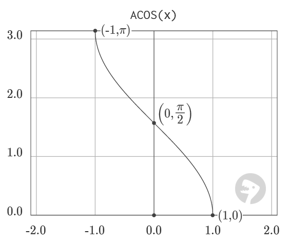
The graph of ACOS visualizes the output of the function in the range from -1 to 1. ACOS is the inverse of the COS function. However, because COS is a periodic function, the output of ACOS is limited to the range from 0 to π.
Graph courtesy of wumbo.net .
