Two

Explanation

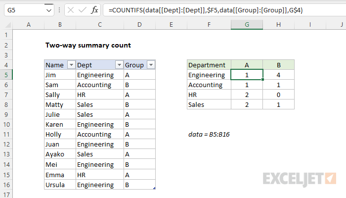
In this example, the goal is to count the people shown in the table by both Department (Dept) and Group as shown in the worksheet. A simple way to do this is with the COUNTIFS function.

COUNTIFS function

The COUNTIFS function is designed to count things based on more than one condition. Conditions are supplied to COUNTIFS in range/criteria “pairs” like this:

=COUNTIFS(range1,criteria1,range2,criteria2)

In this problem, the first step is to create the shell of the summary table that contains one set of criteria in the left-most column, and the second set of criteria in the top row as column headers like this:

The next step is to enter the COUNTIFS function in cell G5 with the first condition for Department:

=COUNTIFS(dept,$F5

For criteria_range1 , we use the named range dept (B5:B16). For criteria1 , we use the mixed reference $F5. Cell F5 contains the value “Engineering”, which will be used for criteria. We use a mixed reference to lock the column only so that the formula will still refer to column F when we copy it to the next column. We leave the row relative because we want the row to change as we copy the formula down. Note that a named range automatically behaves like an absolute reference , so we don’t need to do anything special with the range; it will not change when copied.

Next, we enter the second range/criteria pair to target values for Group:

=COUNTIFS(dept,$F5,group,G$4)

For criteria_range2 , we use the named range group (C5:C16). For criteria2 , we use the mixed reference G$4. Cell G4 contains the value “A”, which will be used for criteria. We use a mixed reference to lock the row only so that the formula will still refer to row 4 when we copy it down.

This is the final formula entered in cell G5, and copied into the range G5:H8. To recap, the named ranges dept and group automatically behave like absolute references and will not change. The references to $F5 and G$4 however are mixed. As the formula is copied, the row in $F5 changes and the column in G$4 changes, which allows the COUNTIFS function to generate correct counts for all combinations of Department and Group.

Excel Table option

When you use an Excel Table to hold source data, you get some nice benefits, including a table that automatically expands when rows are added. Excel Tables use structured references , which appear automatically in formulas that refer to them. In the screen below, the formula in G5 is:

=COUNTIFS(data[[Dept]:[Dept]],$F5,data[[Group]:[Group]],G$4)

This formula is a bit more complex than usual, because the Dept and Group columns need to be locked in a special way with the double square brackets and a colon to allow the formula to be copied across the summary tabled. The two references below show this difference in syntax:

data[Dept] // normal
data[[Dept]:[Dept]] // locked

For more on Excel Tables and structured references, see the videos below. One of the videos shows an easy way to lock a structured reference. If you are new to Excel Tables, see What is an Excel Table ?

Dynamic array option

In the latest version of Excel, which supports dynamic array formulas , you can adapt this example to automatically extract the values for Dept and Group with the UNIQUE function . If fact, if we throw in the LET function and two new functions, HSTACK and VSTACK , it is possible to write a single all-in-one formula that builds a complete summary table like this:

=LET(
  depts,UNIQUE(data[Dept]),
  groups,TRANSPOSE(UNIQUE(data[Group])),
  counts,COUNTIFS(data[Dept],depts,data[Group],groups),
  HSTACK(VSTACK({"Department"},depts),VSTACK(groups,counts))
)

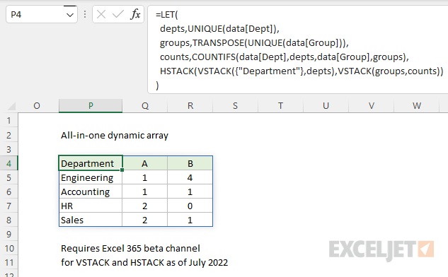
Note: VSTACK and HSTACK are still in beta, available via the Beta Channel for Excel 365.

The best thing about this approach is that any changes to the source data will be reflected in the summary table instantly, with no need to refresh or edit the formula. As a bonus, there is no need to lock specific cell references. The formula above is a great example of how dynamic array formulas will completely change formula solutions in the future. See this example for another related problem with a more complete walkthrough.

Explanation

In this example, the goal is to calculate a running total in column D of the worksheet as shown. A running total, or cumulative sum, is a set of partial sums that changes as more data is collected. Each calculation represents the sum of values up to that point. In this example, each calculation takes into account another month of the year. There are several ways to approach this problem, as explained below.

Note: if you want to create a running total in an Excel Table , you’ll want to take a different approach from the formulas below. See this example .

SUM with expanding range

An easy way to create a running total in Excel is to use the SUM function with what is called an " expanding reference " — a special kind of reference that includes both absolute and relative parts. In the example shown, the formula in D5 is:

=SUM($C$5:C5)

Notice this range refers to one cell only (C5:C5). However, while the first reference to C5 on the left side of the colon (:) is an absolute reference ($C$5), the second reference is a relative reference (C5). As a result, when the formula is copied down the column, the left side of the range is “locked” and won’t change, but the right side of the range is relative and will change at each new row. The result is that the range expands by one row each time it is copied down:

=SUM($C$5:C5) // formula in D5
=SUM($C$5:C6) // formula in D6
=SUM($C$5:C7) // formula in D7
=SUM($C$5:C8) // formula in D8

At each new row, the SUM function receives a larger range that includes the amount in the current row. The result is a cumulative sum of the values in column C up to that point.

Note: formulas with expanding ranges can cause performance problems in large sets of data. The formula below is more efficient.

SUM with two values

Another nice way to solve this problem is to use the SUM function to add the current amount to the previous cumulative sum. In cell D5, you can write a formula like this:

=SUM(C5,D4)

You can see this option in the screen below:

This may seem unusual, since D4 contains text, and not a number. However, the purpose of constructing the formula this way is to allow the same formula to be copied down the column without changes. Using the same formula in a column is considered a best practice because it makes things more consistent and reduces the chance of errors when formulas are copied. The reason we use the SUM function in this formula, instead of simple addition, is that SUM will automatically ignore text values . If we try instead to write a formula like this:

=C5+D4 // returns #VALUE!

The result is a #VALUE! error, because Excel’s formula engine by default will not allow a number and text to be added together.

SCAN function

This problem can also be solved with the SCAN function , a new function in Excel designed to work with dynamic arrays . SCAN can be used to generate running totals and other calculations that show intermediate or incremental results. The SCAN function uses the LAMBDA function to apply the logic needed. The LAMBDA is applied to each value, and the result from SCAN is an array of results with the same dimensions as the original array. The structure of the LAMBDA used inside SCAN looks like this:

LAMBDA(a,v,calculation)

The first argument, a , is the accumulator used to create intermediate values. The accumulator begins as the initial_value provided to SCAN and changes as the SCAN function loops over the elements in array and applies a calculation. The v argument represents the value of each element in array . Calculation is the formula that creates the intermediate values that will appear in the final result. In this example, the basic SCAN formula to create a running total looks like this:

=SCAN(0,C5:C16,LAMBDA(a,v,a+v))

Notice the initial value of the accumulator is zero. At each new row, we simply add the current value (v) to the accumulator (a). Because we give SCAN an array that contains 12 values, SCAN will return an array with 12 results like this:

{1000;3500;5250;9750;15950;21450;25700;25700;25700;25700;25700;25700}

All twelve values will spill into the range D5:D16. To skip rows where the value in column C is not yet available, we can adapt the formula as follows:

=SCAN(0,C5:C16,LAMBDA(a,v,IF(v<>"",a+v,"")))

In this version, we check to see if the current value (v) is not empty . If so, we return a+v. If v is empty, we return an empty string (""). The array returned by SCAN with the modified LAMBDA looks like this:

{1000;3500;5250;9750;15950;21450;25700;"";"";"";"";""}

Here is the result on the worksheet:

Notice the last five values are empty strings, which will display as blank cells in Excel. The key advantage to use SCAN in a problem like this is that it returns all results at the same time in a dynamic array . This makes it possible to use SCAN in more powerful all-in-one formulas .

Pivot Table

A Pivot Table is another good way to calculate running totals. See a basic example here .