Explanation
The SUMIFS function is designed to sum numeric values using multiple criteria. In the example shown, the data in the range B5:E15 shows a sales pipeline where each row is an opportunity owned by a salesperson, at a specific stage. The formula in H5 is:
=SUMIFS(value,name,$G5,stage,H$4)
The first part of the formula sums opportunities by salesperson:
=SUMIFS(value,name,$G5 // sum by name
- Sum range is the named range values
- Criteria range 1 is the named range name
- Criteria 1 comes from cell G5
Notice $G5 is a mixed reference , with the column locked and the row relative. This allows the formula to change as needed when the formula is copied throughout the table.
The next range/criteria pair in SUMIFS, sums by stage:
stage,H$4 // sum by stage
- Criteria range 2 is the named range stage
- Criteria 2 is H$4
Again, H$4 is a mixed reference, with the column relative and the row locked. This allows the criteria to pick up the stage values in row 4 as the formula is copied across and down the table.
With both criteria together, the SUMIFS function correctly sums the opportunities by name and by stage.
Without names ranges
This example uses named ranges for convenience only. Without named ranges, the equivalent formula is:
=SUMIFS($C$5:$C$15,$B$5:$B$15,$G5,$D$5:$D$15,H$4)
Notice references for name, value, and stage are now absolute references to prevent changes as the formula is copied across and down the table.
Note: a pivot table would also be an excellent way to solve this problem.
Explanation
A circular reference occurs when a formula refers directly to its own cell, or refers to another cell that depends on the original cell. This creates an infinite loop that cannot be resolved. For example, if cell A1 contains a formula that refers to B1, and B1 contains a formula that refers to A1, this creates a circular reference. Circular reference errors are not like other errors in Excel in that they don’t display on the worksheet and don’t have a numeric error code. To find circular references, navigate to Formulas > Error checking > Circular references.
Example
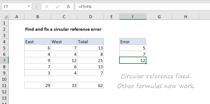
In the worksheet shown, the formula in F7 is:
=F5+F6+F7
This creates a circular reference because the formula, entered in cell F7, refers to F7. This in turn throws off other formula results in D7, C11, and D11:
=F7 // formula in C7
=SUM(B7:C7) // formula in D7
=SUM(C5:C9) // formula in C11
=SUM(D5:D9) // formula in D11
Circular references can cause many problems (and a lot of confusion) because they may cause other formulas to return zero, or a different incorrect result.
The circular reference error message
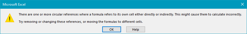
When a circular reference occurs in a spreadsheet, you’ll see a warning like this:
“There are one or more circular references where a formula refers to its own cell either directly or indirectly. This might cause them to calculate incorrectly. Try removing or changing these references, or moving the formulas to different cells.”
This warning will appear sporadically while editing, or when a worksheet is opened.
Finding and fixing circular references
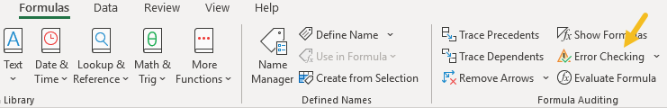
To resolve circular references, you’ll need to find the cell(s) with incorrect cell references and adjust as needed. However, unlike other errors (#N/A, #VALUE!, etc.) circular references don’t appear directly in the cell. To find the source of a circular reference error, use the Error Checking menu on the Formulas tab of the ribbon.
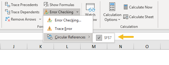
Select the Circular References item to see the source of circular references:
Below, the circular reference has been fixed and other formulas now return the correct results: