Purpose
Return value
Syntax
=VALUETOTEXT(value,[format])
- value - The value to convert to text.
- format - [optional] Output format. 0 = concise (default), and 1 = strict.
Using the VALUETOTEXT function
The VALUETOTEXT function converts a value to a text string . By default, text values pass through unaffected. However, in strict mode, text values are enclosed in double quotes (""). VALUETOTEXT will always remove number formatting applied to numeric values, regardless of format .
The VALUETOTEXT function takes two arguments: value and format . Value is the value to convert to text. The format argument controls the structure of the output. By default, format is zero and VALUETOTEXT will output a “concise” format text value, essentially the normal format that Excel will use to display any text value. When format is set to 1 (strict format), text values will be enclosed in double quotes ("").
VALUETOTEXT is related to the ARRAYTOTEXT function , which performs the same kind of text conversion on arrays .
With numeric values
With the value 100 in cell A1:
=VALUETOTEXT(A1) // returns "100"
=VALUETOTEXT(A1,0) // returns "100"
=VALUETOTEXT(A1,1) // returns "100"
In all cases, 100 is returned as a normal text string, and you will not see double quotes ("") in the output on a worksheet. However, you will see the output aligned left in cells with the General number format applied, since text values appear aligned left in Excel by default. If any number formatting (i.e. currency, percentage, etc.) has been applied to cell A1, it will be lost in the conversion.
With text values
With the text “apple” in cell A1:
=VALUETOTEXT(A1) // returns "apple"
=VALUETOTEXT(A1,0) // returns "apple"
=VALUETOTEXT(A1,1) // returns ""apple""
Notice in the first two examples above, the text “apple” passes through unchanged. In the third example, where format is set to 1 (strict), double quotes are added to the text and will display on the worksheet.
Purpose
Return value
Syntax
=VSTACK(array1,[array2],...)
- array1 - The first array or range to combine.
- array2 - [optional] The second array or range to combine.
Using the VSTACK function
The Excel VSTACK function combines arrays vertically into a single array. Each subsequent array is appended to the bottom of the previous array. The result from VSTACK is a single array that spills onto the worksheet into multiple cells.
VSTACK works equally well for ranges on a worksheet or in-memory arrays created by a formula. The output from VSTACK is fully dynamic. If data in the given arrays changes, the result from VSTACK will immediately update. VSTACK works well with Excel Tables , as seen in the worksheet above, since Excel Tables automatically expand when new data is added.
Use VSTACK to combine ranges vertically and HSTACK to combine ranges horizontally.
Basic usage
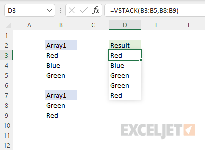
VSTACK stacks ranges or arrays vertically. In the example below, the range B3:B5 is combined with the range B8:B9. Each subsequent range/array is appended to the bottom of the previous range/array. The formula in D3 is:
=VSTACK(B3:B5,B8:B9)
Range with array
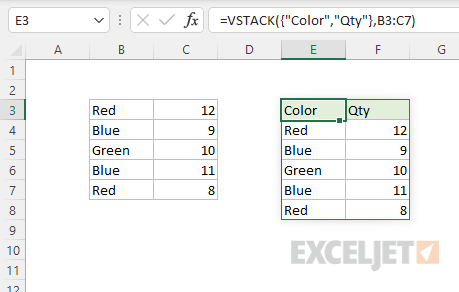
VSTACK can work interchangeably with both arrays and ranges. In the worksheet below, we combine the array constant {“Color”,“Qty”} with the range B3:C7. The formula in E3 is:
=VSTACK({"Color","Qty"},B3:C7)
Arrays of different size
When VSTACK is used with arrays of different size, the smaller array will be expanded to match the size of the larger array. In other words, the smaller array is “padded” to match the size of the larger array, as seen in the example below. The formula in cell E5 is:
=VSTACK(B5:C8,B11:B13)
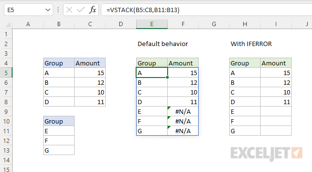
By default, the cells used for padding will display the #N/A error. One option for trapping these errors is to use the IFERROR function . The formula in H5 is:
=IFERROR(VSTACK(B5:C8,B11:B13),"")
In this formula IFERROR is configured to replace errors with an empty string (""), which displays as an empty cell.
