Explanation
When VLOOKUP can’t find a value in a lookup table, it returns the #N/A error. In this example, the goal is to remove the #N/A error that VLOOKUP returns when it can’t find a lookup value. In general, the best way to do this is to use the IFNA function. However, the IFERROR function can also be used in the same way. Both options are explained below.
VLOOKUP function
The VLOOKUP function performs a lookup operation on vertical data. The generic syntax for VLOOKUP looks like this:
VLOOKUP(A1,table,column,FALSE)
Where A1 contains a value to lookup, table is the data, column is a number, and FALSE specifies exact match, which is required in this example. In the workbook shown, we want to enter an abbreviation in cell E5 and get the correct State name in cell F5, where all data is in an Excel Table named data . To do this, we can use VLOOKUP in a formula like this:
VLOOKUP(E5,data,2,FALSE)
When a valid 2-letter code is entered in cell E5, VLOOKUP will return the corresponding State. For example, if “CA” is entered in cell E5, VLOOKUP will return “California”:
VLOOKUP("CA",data,2,FALSE) // returns "California"
If an invalid code is entered in cell E5, VLOOKUP will return an #N/A error:
VLOOKUP("XX",data,2,FALSE) // returns #N/A
The screen below shows how this error looks on the worksheet:

The #N/A error technically means “not available”. However, you may want to return a more friendly result. You can do this by combining VLOOKUP with the IFNA function.
VLOOKUP with IFNA
The IFNA function is a simple way to trap and handle #N/A errors without catching other errors. When used with a formula, the generic syntax looks like this:
=IFNA(formula,alternative)
Here, the formula might return a #N/A error; the alternative is the value or formula to return in that case. To trap the #N/A error in this example, we wrap the IFNA function around the original VLOOKUP function and provide an alternate value. For example, to return “Not found” when VLOOKUP returns #N/A, we can use a formula like this:
=IFNA(VLOOKUP(E5,data,2,FALSE),"Not found")
Now, when VLOOKUP returns the #N/A error, IFNA takes over and returns “Not found”:
=IFNA(VLOOKUP("XX",data,2,FALSE),"Not found") // returns "Not found"
To return a different message, just change the second argument in IFNA:
=IFNA(VLOOKUP("XX",data,2,FALSE),"Invalid code") // returns "Invalid code"
If you would prefer to return nothing, you can provide an empty string ("") instead, like this:
=IFNA(VLOOKUP("XX",data,2,FALSE),"") // returns ""
The result from this formula will look like an empty cell when the lookup Code is not found.
VLOOKUP with IFERROR
You can also trap #N/A errors returned by VLOOKUP with the IFERROR function like this:
=IFERROR(VLOOKUP(E5,data,2,FALSE),"Not found")
IFERROR works just like the IFNA function — it catches an #N/A error returned by VLOOKUP and returns an alternative result. The difference is that IFERROR will catch other errors as well.
The #N/A error is Excel’s way of telling you a value was not found. With the more general IFERROR function, there is a risk that you might catch other unrelated errors and return a confusing result. For example, if you have a typo in a function name, Excel will return a #NAME! error. Or, if rows/columns are deleted in a worksheet, a formula may return a #REF! error. While IFNA will let these errors come through (so you see them), IFERROR will catch these errors, too, which can hide the underlying problem. For these reasons, I recommend you use the IFNA function when the purpose is to trap #N/A errors only.
Older versions of Excel
In earlier versions of Excel that lack the IFNA function, you will need to repeat the VLOOKUP inside an IF function that catches an error with the ISNA function . For example:
=IF(ISNA(VLOOKUP(A1,table,2,FALSE)),"Not found",VLOOKUP(A1,table,2,FALSE))
Explanation
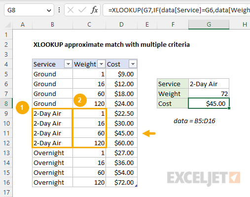
In this example, the goal is to look up the correct shipping cost for an item based on the shipping service selected and the weight of the item. The challenge is that we also need to filter by service. This means we need to apply criteria in two steps: (1) match based on Service, and (2) match based on Weight. The screen below shows the basic idea:
One way to solve this problem is with XLOOKUP + the IF function to perform the required filtering. One reason this works nicely is that the IF function returns 12 results, which correspond to the 12 rows in the table. This means XLOOKUP can return the right value in the table because all 12 rows are still intact. You could instead use the FILTER function , with a bit more configuration. See below for details.
Background reading
This article assumes you are familiar with Excel Tables and XLOOKUP. If not, see:
- Excel Tables - introduction and overview
- XLOOKUP function - overview with examples and videos
Basic XLOOKUP
In XLOOKUP formulas, a lookup_array and return_array are provided as arguments. XLOOKUP locates the lookup value in the lookup array. Then it returns the corresponding value in the return array. If you are new to XLOOKUP, this short video shows a basic example.
Looking at this problem from the inside out, the core of the solution is an approximate match lookup based on weight. To illustrate, the screen below shows a simplified version of the same problem with the Service removed:

The formula in cell F5 is:
=XLOOKUP(F4,B5:B8,C5:C8,,-1)
The lookup_array is the weight in the range B5:B8, and the return_array is the cost in the range C5:C8. Notice the match_mode argument inside XLOOKUP is set to -1, to find the largest value in B5:B8 that is less than or equal to the lookup value in cell F4. In this case, the largest value less than or equal to 72 is 60, so XLOOKUP matches the 60 and returns $18.00 as a final result:
=INDEX(C5:C8,3) // returns 18
So far, so good. We have a simple working XLOOKUP formula that returns the correct cost based on an approximate match lookup. The challenge is that we also need to match based on the Service. To do that, we need to extend the formula to handle another condition.
Adding criteria for service
We know how to look up costs based on weight. The remaining challenge is that we also need to take into account the Service. For simple exact-match scenarios, we can use Boolean logic , as explained here . But in this example, we need to perform an approximate match , so using Boolean logic will not work well. Another approach is to “filter out” extraneous entries in the table so we are left only with entries that correspond to the Service we are looking up. The classic way to do this is with the IF function . This is the approach used in the example shown, where the formula in cell G8 is:
=XLOOKUP(G7,IF(data[Service]=G6,data[Weight]),data[Cost],,-1)
The filtering is done with the IF function, which appears inside the XLOOKUP function like this:
IF(data[Service]=G6,data[Weight])
This code tests the values in the Service column to see if they match the value in G6. Where there is a match, the corresponding values in with Weight column are returned. If there is no match, the IF function returns FALSE. Because there are 12 rows in the table, the IF function returns an array that contains 12 results like this:
{FALSE;FALSE;FALSE;FALSE;1;16;60;120;FALSE;FALSE;FALSE;FALSE}
Notice the only weights that remain in the array are those that correspond to the “2-Day-Air” service; all other weights have been replaced with FALSE. You can visualize this operation in the original data as shown below:

This array is delivered directly to XLOOKUP as the lookup_array:
=XLOOKUP(G7,{FALSE;FALSE;FALSE;FALSE;1;16;60;120;FALSE;FALSE;FALSE;FALSE},data[Cost],,-1)
With a weight of 72 in cell G7, XLOOKUP matches 60 and returns $45.00 as the final result. Notice that we are using -1 inside XLOOKUP as the match_mode argument. This will cause XLOOKUP to match a value that is less than or equal to the lookup value.
XLOOKUP with FILTER
Another way to solve this problem is with XLOOKUP and the FILTER function, like this:
=XLOOKUP(G7,FILTER(data[Weight],data[Service]=G6),FILTER(data[Cost],data[Service]=G6),,-1)
In this formula, we remove data for other services with the FILTER function. Inside XLOOKUP, FILTER creates the lookup_array like this:
FILTER(data[Weight],data[Service]=G6) // returns {1;16;60;120}
The return_array is created in the same way:
FILTER(data[Cost],data[Service]=G6) // returns {22.5;30;45;60}
After FILTER runs, XLOOKUP is only working with values associated with the 2-Day air service:
=XLOOKUP(G7,{1;16;60;120},{22.5;30;45;60},,-1)
With 72 in cell G7, XLOOKUP returns the same result as before, a cost of $45.00. This formula works nicely and is perhaps more intuitive than XLOOKUP + IF. However, the tradeoff is a more complex formula since FILTER must be used twice.
