Purpose
Return value
Syntax
=VSTACK(array1,[array2],...)
- array1 - The first array or range to combine.
- array2 - [optional] The second array or range to combine.
Using the VSTACK function
The Excel VSTACK function combines arrays vertically into a single array. Each subsequent array is appended to the bottom of the previous array. The result from VSTACK is a single array that spills onto the worksheet into multiple cells.
VSTACK works equally well for ranges on a worksheet or in-memory arrays created by a formula. The output from VSTACK is fully dynamic. If data in the given arrays changes, the result from VSTACK will immediately update. VSTACK works well with Excel Tables , as seen in the worksheet above, since Excel Tables automatically expand when new data is added.
Use VSTACK to combine ranges vertically and HSTACK to combine ranges horizontally.
Basic usage
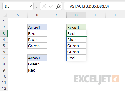
VSTACK stacks ranges or arrays vertically. In the example below, the range B3:B5 is combined with the range B8:B9. Each subsequent range/array is appended to the bottom of the previous range/array. The formula in D3 is:
=VSTACK(B3:B5,B8:B9)
Range with array
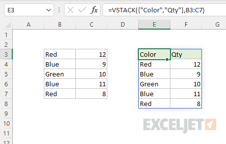
VSTACK can work interchangeably with both arrays and ranges. In the worksheet below, we combine the array constant {“Color”,“Qty”} with the range B3:C7. The formula in E3 is:
=VSTACK({"Color","Qty"},B3:C7)
Arrays of different size
When VSTACK is used with arrays of different size, the smaller array will be expanded to match the size of the larger array. In other words, the smaller array is “padded” to match the size of the larger array, as seen in the example below. The formula in cell E5 is:
=VSTACK(B5:C8,B11:B13)
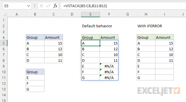
By default, the cells used for padding will display the #N/A error. One option for trapping these errors is to use the IFERROR function . The formula in H5 is:
=IFERROR(VSTACK(B5:C8,B11:B13),"")
In this formula IFERROR is configured to replace errors with an empty string (""), which displays as an empty cell.
Purpose
Return value
Syntax
=WRAPCOLS(vector,wrap_count,[pad_with])
- vector - The array or range to wrap.
- wrap_count - Max values in each column.
- pad_with - [optional] Value to use for unfilled places.
Using the WRAPCOLS function
The WRAPCOLS function converts a one-dimensional array into a two-dimensional array by wrapping values into separate columns. The length of each column is given as the wrap_count argument: when the count is reached, WRAPCOLS starts a new column.
The WRAPCOLS function takes three arguments: vector , wrap_count , and pad_with . Vector and wrap_count are both required. Vector must be a one-dimensional array or range. Wrap_count is a number that represents the length of each column. The final argument, pad_with , is an optional value to use if there are empty spots in the last column. If no value is supplied for pad_with, WRAPCOLS will return an #N/A error after all values in vector have been used. You can override this behavior by providing a custom value for the pad_with argument.
Basic usage
WRAPCOLS outputs values “by column”, working top to bottom, left to right. When wrap_count has been reached, WRAPCOLS starts a new column. In the worksheet below, the goal is to wrap the range C2:J2 into columns that each contain 4 values. The formula in B5 is:
=WRAPCOLS(C2:J2,4)
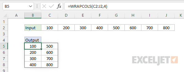
Notice WRAPCOLS outputs values by column, top to bottom, and each column contains 4 rows.
Wrap count
Wrap_count represents the maximum number of values in each column. Once the count has been reached, WRAPCOLS starts a new column. In the screen below, you can see how this works. The formula in D3 uses a wrap_count of 3:
=WRAPCOLS(B3:B14,4)
The formula in D10 uses a wrap_count of 4:
=WRAPCOLS(B3:B14,3)
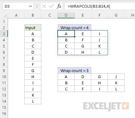
Notice values are output top to bottom.
Padding
If no value is supplied for pad_with, WRAPCOLS will return an #N/A error after all values in the source array have been accounted for. You will see these errors appear in the last column when the total number of items in the source array is not evenly divisible by the wrap_count . You can override this behavior by providing a custom value for the pad_with argument. The formula in D3 shows default behavior. No value for pad_with has been provided:
=WRAPCOLS(B3:B12,4)
The input range contains only 10 cells, which is not evenly divisible by a wrap_count of 4. As a result, the last 2 cells return #N/A. The formula in D10 supplied “x” for pad_with:
=WRAPCOLS(B3:B12,4,"x")
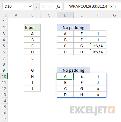
Notice the #N/A errors have been replaced by “x” in the resulting array.
Notes
- WRAPCOLS will return a #VALUE! error if vector is not a one-dimensional array or range.
- Wrap_count indicates the size of each column not the number of columns.
