Explanation
In this example, the goal is to calculate a weighted average of scores for each name in the table using the weights that appear in the named range weights (I5:K5) and the scores in columns C through E. A weighted average (also called a weighted mean ) is an average where some values are more important than others. In other words, some values have more “weight”. We can calculate a weighted average by multiplying the values to average by their corresponding weights, then dividing the sum of results by the sum of weights. In Excel, this can be represented with the generic formula below, where weights and values are cell ranges:
=SUMPRODUCT(weights,values)/SUM(weights)
The core of this formula is the SUMPRODUCT function. In a nutshell, SUMPRODUCT multiplies ranges or arrays together and returns the sum of products. This sounds really boring, but SUMPRODUCT is an incredibly versatile function that shows up in all kinds of useful formulas. See this page for an overview.
Worksheet example
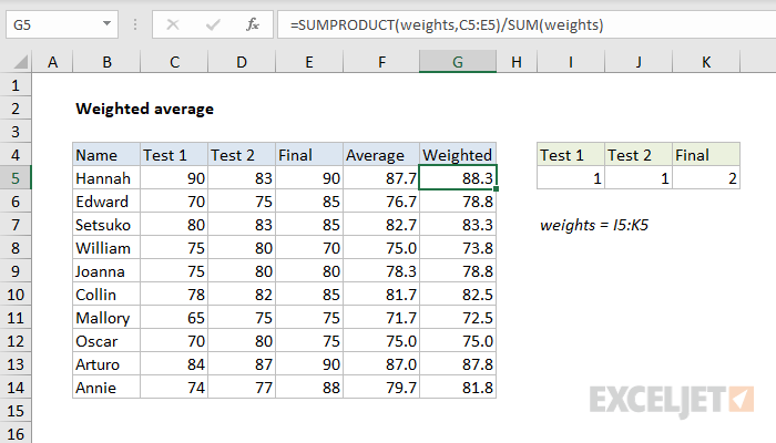
In the worksheet shown, scores for 3 tests appear in columns C through E, and weights appear in the named range weights (I5:K5). The formula in cell G5 is:
=SUMPRODUCT(weights,C5:E5)/SUM(weights)
Looking first at the left side, we use the SUMPRODUCT function to multiply weights by corresponding scores and sum the result:
=SUMPRODUCT(weights,C5:E5) // returns 88.25
SUMPRODUCT multiplies corresponding elements of the two arrays together, then returns the sum of the product. We can visualize this operation in cell G5 like this:
=SUMPRODUCT({0.25,0.25,0.5},{90,83,90})
=SUMPRODUCT({22.5,20.75,45})
=88.25
The result is then divided by the sum of the weights:
=88.25/SUM(weights)
=88.25/SUM({0.25,0.25,0.5})
=88.25/1
=88.25
Note: when calculating a weighted average, it is common to assign weights that add up to the number 1. As you can see above, when the weights do add up to 1, the denominator becomes 1 and has no effect in the formula. However, it is not required that weights add up to 1, and the general form of the formula used above is meant to handle either case. See below for an example where weights do not add up to 1.
As the formula is copied down column G, the named range weights I5:K5 does not change, since it behaves like an absolute reference . However, the scores in C5:E5, which are relative reference , change with each new row. The result is a weighted average for each name in the list as shown. For easy reference, the average in column F is calculated normally with the AVERAGE function :
=AVERAGE(C5:E5)
Weights that do not sum to 1
In the example above, the weights are configured to add up to 1, so the divisor is 1, and the final result is the value returned by SUMPRODUCT. However, a nice feature of the formula is that the weights don’t need to add up to 1. For example, we could use a weight of 1 for the first two tests and a weight of 2 for the final (since the final is twice as important) and the weighted average will be the same:
In cell G5, the formula is solved like this:
=SUMPRODUCT(weights,C5:E5)/SUM(weights)
=SUMPRODUCT({1,1,2},{90,83,90})/SUM(1,1,2)
=SUMPRODUCT({90,83,180})/SUM(1,1,2)
=353/4
=88.25
Note: the values in curly braces {} above are arrays , which map directly to ranges in Excel.
Transposing weights
The SUMPRODUCT function requires that array dimensions be compatible to run correctly. For example, if the data is in a horizontal array , the weights should also be in a horizontal array. If dimensions are not compatible, SUMPRODUCT will return a #VALUE error. To prevent this problem, you may need to transpose the weights to match the data. In the example below, the weights are the same as the original example above, but they are listed in a vertical range:
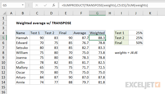
In this case, to calculate a weighted average with the same formula, we need to “flip” the weights into a horizontal array with the TRANSPOSE function like this:
=SUMPRODUCT(TRANSPOSE(weights),C5:E5)/SUM(weights)
After TRANSPOSE runs, the vertical array:
=TRANSPOSE({0.25;0.25;0.5}) // vertical array
becomes a horizontal array like this:
={0.25,0.25,0.5} // horizontal array
Note the semicolons are now commas, which indicate a horizontal array. From this point, the formula is solved the same way as explained earlier.
Explanation
In this example the goal is to return rows in the range B5:E15 that have a specific state value in column E. To make the example dynamic, the state is a variable entered in cell H4. When the state in H4 is changed, the formula should return a new set of records. This is a perfect application for the FILTER function, which is designed to return values that meet specific logical criteria from a set of data.
FILTER function
The FILTER function “filters” a range of data based on supplied criteria. In other words, the FILTER function will extract matching records from a set of data by applying one or more logical tests . The result is an array of matching values from the original data. The FILTER function takes three arguments , and the generic syntax looks like this:
=FILTER(array,include,[if_empty])
In this problem, array is given as B5:E15, which contains the full set of data without headers:
=FILTER(B5:E15,
The include argument is an expression that runs a simple test for matching states:
E5:E15=H4 // test state values
Placing this expression into FILTER as the second argument, we have:
=FILTER(B5:E15,E5:E15=H4,
Finally, the optional if_empty argument is set to “not found” in case no matching data is found:
=FILTER(B5:E15,E5:E15=H4,"not found")
Note the value for if_empty is a text string in double quotes (""). You can customize this message as you like. Supply an empty string ("") to display nothing. If you omit if_empty altogether, FILTER will return a #CALC! error when no data is returned.
When the formula above is entered, the include argument is evaluated. Since there are 11 cells in the range E5:E11 and the value in H4 is “TX”, the include expression returns an array of 11 TRUE and FALSE like this:
{TRUE;FALSE;FALSE;TRUE;FALSE;FALSE;FALSE;FALSE;FALSE;TRUE;TRUE}
Notice the TRUE values in this array correspond to records in the data where the State is “TX”. This array is used by the FILTER function to retrieve matching data. Only rows where the result is TRUE make it into the final output.
Other fields and criteria
Other fields can be filtered in a similar way. For example, to filter the same data on orders that are greater than $100, you can use FILTER like this:
=FILTER(B5:E15,C5:C15>100,"not found")
You can also configure the logic inside the include argument to apply more complex criteria .
