Some older Excel functions don’t spill when you give them a range as input. This article explains why this happens, which functions are affected, and how to fix it.
- Dynamic Arrays and Spilling
- The spilling problem explained
- The simple solution
- List of affected functions
- Why the plus sign?
There are other reasons why a formula might not spill. This article focuses on one specific case: a specific group of older functions that will not accept a range in place of a single value.
Dynamic Arrays and Spilling
In 2019, the Excel team began to introduce dynamic array formulas , a new way to work with data in Excel. In a nutshell, dynamic array formulas can process more than one value at the same time, then return multiple values to the worksheet in a behavior known as " spilling “. Many newer dynamic array functions spill multiple values natively. Good examples are functions like FILTER , SORT , SEQUENCE , and UNIQUE . However, older Excel functions will also spill through a process called " lifting “. When you give a range or array to a function not programmed to accept arrays natively, Excel will “lift” the function and call it multiple times, once for each value in the array. For example, the LEN function is designed to return the number of characters in a text string. If we give LEN the text “apple”, it will return 5:
=LEN("apple") // returns 5
If we give LEN three text strings in an array , it returns an array with three counts, one for each text string:
=LEN({"apple";"banana";"pear"}) // returns {5;6;4}
You can see an example of this in the following worksheet, where the formula in cell D8 looks like this:
=LEN(B8:B10) // returns {5;6;4}
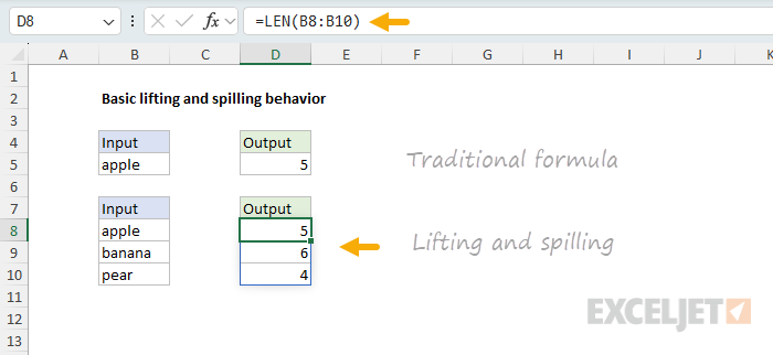
The main thing to understand is that lifting is a built-in behavior that happens automatically. When you give a function more than one value as an input, you will get back multiple results that spill onto the worksheet. It just works. Except when it doesn’t 🙃
The spilling problem explained
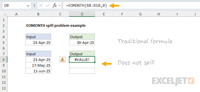
As it turns out, some functions don’t spill when you give them a range instead of a single cell reference. A good example is the EOMONTH function , which returns the last day of the month for any given date. If we give EOMONTH the date 23-Apr-2025, with an offset of 0, it will return the last day of that month, which is 30-Apr-2025. You can see this in the following worksheet, where the formula in cell D5 looks like this:
=EOMONTH(B5,0) // returns 30-Apr-2025
However, if we give EOMONTH a range of three dates, it refuses to spill and instead returns a #VALUE! error with a formula like this in cell D8:
=EOMONTH(B8:B10,0) // returns #VALUE!
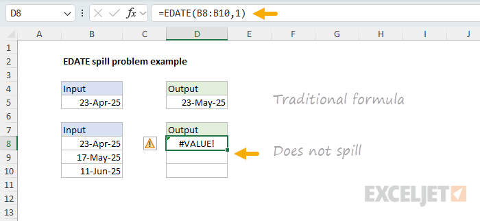
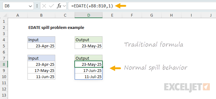
We can see exactly the same problem with the EDATE function , which returns the date a given number of months before or after a given date. If we give EDATE the date 23-Apr-2025, with an offset of 1, it will return the date 23-May-2025. You can see this in the following worksheet, where the formula in cell D5 looks like this:
=EDATE(B5,1) // returns 23-May-2025
However, if we give EDATE a range of three dates, it refuses to spill and instead returns a #VALUE! error with a formula like this in cell D8:
=EDATE(B8:B10,1) // #VALUE! error
What’s going on here? The problem is that some older functions like EOMONTH “resist” spilling when provided a range. This limitation comes from these functions expecting a single cell value instead of a range. The #VALUE! error is essentially reporting the range as an unexpected value. Other common functions that have this same limitation include EDATE, ISEVEN , ISODD , YEARFRAC , WORKDAY , and WORKDAY.INTL . See below for a larger list of affected functions.
The simple solution
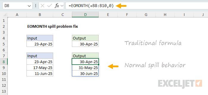
Although this seems like a difficult technical problem, the solution is actually quite simple. The trick is to add a plus sign (+) before the range. This forces Excel to evaluate the range before the function runs. The result is an array of values, which are then passed to the function so that lifting and spilling occur as expected. You can see this fix in the following worksheet, where the formula in cell D8 looks like this:
=EOMONTH(+B8:B10,0) // spills normally
We can do exactly the same thing with the EDATE function, and it will spill normally:
=EDATE(+B8:B10,1) // spills normally
Note: In simple situations like those described above, diagnosing the spill problem and fixing it is fairly straightforward as long as you know about this issue and how to fix it. Where it gets more complicated is when you use a function that resists spilling with a range inside a larger formula. Then, function will return a #VALUE! error that blows up the entire formula, but it will not be so easy to understand what the problem is, since you aren’t actually seeing a function fail to spill on a worksheet.
List of affected functions
The origins of this problem are murky, and it is difficult to find good documentation for Excel functions from the era in which most of these functions were introduced. However, based on conversations with other Excel MVPs, I believe that functions with this spilling limitation all originate from the same development effort: the Analysis ToolPak, which was initially included in Excel 97 as a separate add-in, and later rolled into the core application in Excel 2007. Here is a list of the functions that started life in the Analysis ToolPak:
| Category | Functions |
|---|---|
| Financial | ACCRINT , ACCRINTM , AMORDEGRC , AMORLINC , COUPDAYBS , COUPDAYS , COUPDAYSNC , COUPNCD , COUPNUM , COUPPCD , CUMIPMT * , CUMPRINC , DISC , DOLLARDE , DOLLARFR , DURATION , EFFECT , FVSCHEDULE , INTRATE , MDURATION , NOMINAL , ODDFPRICE , ODDFYIELD , ODDLPRICE , ODDLYIELD , PMT * , PRICE , PRICEDISC , PRICEMAT , RECEIVED , TBILLEQ , TBILLPRICE , TBILLYIELD , XIRR * , XNPV , YIELD , YIELDDISC , YIELDMAT |
| Engineering | BESSELI, BESSELJ, BESSELK, BESSELY, BIN2DEC , BIN2HEX , BIN2OCT , COMPLEX , CONVERT , DEC2BIN , DEC2HEX , DEC2OCT , DELTA , ERF, ERFC, GESTEP, HEX2BIN , HEX2DEC , HEX2OCT , IMABS , IMAGINARY , IMARGUMENT , IMCONJUGATE , IMCOS , IMDIV , IMEXP , IMLN , IMLOG10 , IMLOG2 , IMPOWER , IMPRODUCT * , IMREAL , IMSIN , IMSQRT , IMSUB , IMSUM * , OCT2BIN , OCT2DEC , OCT2HEX |
| Math & Trig | FACTDOUBLE , GCD * , LCM * , MROUND , MULTINOMIAL * , QUOTIENT , RANDBETWEEN , SERIESSUM, SQRTPI |
| Date & Time | EDATE , EOMONTH , NETWORKDAYS , WEEKNUM , WORKDAY , YEARFRAC |
| Information | ISEVEN , ISODD |
| Text | ASC |
Credit: I put together this list using this page on bettersolutions.com .
I quickly tested all of the functions in the list above. Most of them have the spill problem, but there are a few exceptions, which I’ve marked with an asterisk (*) above. Note also that there are a number of functions derived from the ATP functions above that have the spill problem, including WORKDAY.INTL , NETWORKDAYS.INTL , ERF.PRECISE, and ERFC.PRECISE.
When testing these functions, the basic approach is to provide a range in place of any argument that would normally be provided as a single cell reference. For the above functions, the result is usually a #VALUE! error, with exceptions as noted. When you add the plus (+) sign before the range, the formula should lift and spill, and you should get more than one result, depending on the size of the range provided.
Why the plus sign?
Way back in the 1980s, Lotus 1-2-3 was the dominate spreadsheet application, and it allowed you to start a formula with a plus sign (+) instead of an equal sign (=). When Excel added Lotus compatibility in the 1990s, it accepted that syntax, so users migrating to Excel often typed +A1 or +SUM(B2:B10) , which Excel quietly converted to =+A1 and =+SUM(B2:B10) . In Excel, the extra “+” is ignored; it’s just an identity operator. In Excel, the + operator has no effect on a single value, but it will coerce a range into an array , which sidesteps the legacy scalar (i.e., single value) restriction that creates the spilling problem described in this article.
Researching this was interesting. It helped me understand why you occasionally see the + operator turn up in all kinds of simple formulas. I think the reason is that the people who wrote these formulas learned on Lotus 1-2-3. 🙂 I also think it is a matter of convenience for people who use a 10-key (the numeric keypad on a computer keyboard). I ran into many variations of this comment: When I’m typing on the 10 key, I don’t have to move my hand to start a formula with = .. I just hit + with my pinky and start typing. Excel puts the = in on it’s own. We don’t actually type “=+”.
Summary
Excel’s dynamic array formulas were introduced in Excel 365 starting in 2019. A key feature of dynamic arrays is the ability to process multiple values and return multiple results through " spilling .” While newer functions like FILTER and SORT spill natively, older functions use a process called " lifting, " where Excel automatically calls the function multiple times for each value in an array .
However, certain older functions - primarily those originating from Excel’s Analysis ToolPak - resist spilling when given a range as input. Functions like EOMONTH , EDATE , ISEVEN , ISODD , YEARFRAC , WORKDAY , and WORKDAY.INTL will return a #VALUE! error instead of spilling results because they expect single values rather than ranges.
The solution is simple: add a plus sign (+) before the range reference. For example, =EOMONTH(+A1:A5,1) works where =EOMONTH(A1:A5,1) fails. The + operator forces Excel to evaluate the range first, converting it to an array of values that can then be processed through normal lifting and spilling behavior.
This limitation affects dozens of functions across financial, engineering, math, date/time, and information categories - essentially all functions that were originally part of the Analysis ToolPak add-in.
If you’ve ever had a formula like =A1=B1 return FALSE—even though the values in A1 and B1 seem exactly the same—you’ve run into one of Excel’s most puzzling quirks: the floating-point error. These tiny differences are usually invisible, but they can cause formula checks and even conditional formatting rules to fail in unexpected ways. This article explains why these errors happen, how to spot them, and how to fix them with simple techniques like rounding.
- Why Your Numbers Don’t Add Up
- What Is a Floating Point Error?
- Example 1 - Typical rounding problem
- Example 2 - Floating point errors with subtraction
- Example 3 - Floating point errors with incremental addition
- Set precision as displayed (not recommended)
- Other rounding functions in Excel
- Takeaways
- Floating point details
- Useful Links
Why Your Numbers Don’t Add Up
When working with numbers in Excel, especially when adding or subtracting many values during reconciliation, you may run into small discrepancies that seem illogical, like two totals that should match but don’t. There are two basic reasons why you might run into this situation:
- A simple rounding problem.
- A floating-point error.
The first problem is more common and is often related to Excel’s number formatting or sometimes to the column width. The second problem is less common and more difficult to understand. It happens because Excel uses binary floating-point numbers, which can’t represent some decimal values exactly. As a result, tiny rounding errors accumulate during calculations, creating results that are extremely close but not exactly equal. These differences are often invisible on the worksheet but can cause equality checks or balance comparisons to fail unexpectedly:
- A conditional formatting rule shows a calculated number in red when it should be green.
- A formula that checks a calculation unexpectedly returns FALSE.
- A final balance does not equal the expected result, although it appears to be correct.
This problem is not limited to Excel. Other environments and computer languages have the same limitation.
What Is a Floating Point Error?
Excel uses the decimal number system to display results. This is the base-10 system we use every day, with ten digits (0 through 9) to represent all numbers. In decimal, each digit’s position in a number represents a power of 10, with values increasing from right to left. Computers, however, (including Excel) store numbers using a system called floating-point arithmetic, based on binary (base 2). In binary, only two digits (0 and 1) are used, and each position represents a power of 2. This system is efficient for computation, but it has an important limitation: many decimal values can’t be represented exactly in binary.
For example, numbers like 0.1 and 0.2 can’t be represented perfectly in binary, so Excel stores values like 0.10000000000000001 and 0.20000000000000001 instead. Likewise, 1/3 doesn’t have an exact decimal representation (it becomes 0.3333333…). As a result, when Excel stores these values, it must approximate them. These tiny approximations—called floating-point errors—can cause surprising results when performing calculations or comparisons
Let’s look at some examples, starting with a problem that is not a floating-point error.
Example 1 - Typical rounding problem
Before we get into specific examples of floating-point errors, let’s look at a typical rounding problem. This is not a floating-point error, but rather a misunderstanding created by the way that Excel displays numbers when number formatting is applied. In the worksheet below, we have a list of products in column B and corresponding prices in column C. In column D, we have calculated a 10% discount with a formula like this:
=C5*10%

In column F, we have manually entered the same discount. In column G, we have a formula that checks the calculated discount in column C against the hardcoded discount in column F. The formula in G5 is:
=D5=F5

In all rows, it returns FALSE. What’s going on?
The problem is that the calculated values in column D are not rounded, but they look rounded because a Number format with 2 decimal places has been applied to them. Number formats in Excel change the way a number is displayed, but they do not change the underlying number. If we change that number format to show four decimal places, you can see the problem clearly:

Tip: Another way to see more decimal places, temporarily apply the General number format with the shortcut Ctrl + Shift + ~. Depending on the number, Excel will display up to 9 decimal places if the column is wide enough. Then Ctrl + Z to undo.
The discounts in column D are not rounded, but the number format with 2 decimal places causes them to look rounded. On the other hand, the numbers typed into column F are actually rounded to two decimal places. This is why none of the numbers match. If you need to compare these numbers apples-to-apples in a case like this, a good option is to modify the check formula in G5 like this
=ROUND(D5,2)=F5
This formula uses the ROUND function to round the value in D5 to two decimal places before comparing it to the value in F5. The advantage of this approach is that it leaves the original values in column D unchanged, but still lets you compare to the expected results. With this change, you can see that now the check formula in column E returns TRUE in all rows:

Another option is to round the values in column D right from the start using a formula like this in D5:
=ROUND(C5*10%,2)
This option will actually round the discounts in column D to two decimal places, and they will match the hardcoded values in column F. Both options are valid, but I would generally avoid rounding the discounts unless you have a reason to do so.
To summarize, this is a rounding problem, not a floating-point error. Number formats in Excel can make it appear as though numbers are the same even when they aren’t.
Tip: Avoid rounding too early in your calculations, unless it is required. Early rounding can introduce cumulative errors. Instead, calculate precisely first, then apply rounding only at the final step. This method preserves accuracy.
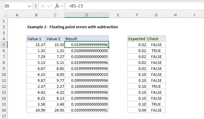
Example 2 - Floating point errors with subtraction
Now let’s look at an example of actual floating-point errors. In the worksheet below, we are subtracting numbers in column C from the numbers in column B. The formula in D5 looks like this:
=B5-C5

The values in columns B and C are ordinary numbers with exactly two decimal places, like dollars and cents. Column D contains the calculated result, and column E contains the expected result (hard-coded). If you look at the numbers in columns B and C, you can probably guess what the result should be. The formula in column F compares the actual result to the expected result, like this:
=D5=E5
As you can see, most of the checks in column G are FALSE, even though we would expect all results to be TRUE. This is quite confusing. The calculation is simple, and the results look perfectly ordinary. What’s going on here? This is a case where some of the numbers in column D can’t be perfectly stored as binary numbers. They look normal, but if we look more carefully, we can find some tiny problems.
The first thing to check is the raw numbers. To show more decimal places, use the keyboard shortcut Ctrl + 1 to open the Format cells dialog box, then navigate to Number and set the decimal places to 16:

Then adjust the column width to show the full value. Now we can see that some of these numbers are not what they appear to be:
Tip: Another way to increase decimal places is to punch the “increase decimal” button on the ribbon 16 times, but I like the Ctrl + 1 method because it’s fast and you can quickly undo with Ctrl+Z after checking the raw number. Note also if you want to check a static number typed or pasted into Excel, the formula bar will show the number in its raw form without number formatting.
Now that we know the problem, how should we fix it? One way to fix a floating-point error in Excel is to add rounding to the appropriate formulas. For example, in this worksheet, we can modify the Check formula to round the value in column D5 before testing. Since we’re working with numbers that are accurate to two decimal places, we can use the ROUND function with num_digits set to 2. You can see this approach in the worksheet below, where the formula in G5 is now:
=ROUND(D5,2)=F5

Another good way to manage floating-point errors is to use a formula that ensures that calculated and expected results are within a specified tolerance. We can use the ABS function to create a tolerance-based check like this:
=ABS(D5-F5)<0.0000000001
We first subtract the expected result from the calculated result. Then we take the absolute value, and check the difference is less than 0.0000000001. This method allows you to bypass rounding entirely, by defining a threshold for how close is “close enough.” You can see this formula in action below:

Note: The tolerance above is very small. In general, you should adjust the tolerance to suit the specific use case.
Example 3 - Floating point errors with incremental addition
Floating-point errors can also appear when you add the same decimal value repeatedly. In the worksheet below, we are repeatedly adding 0.1 to a starting value of -1.9. All values in column B are generated with the SEQUENCE function with this formula in cell B5:
=SEQUENCE(F6,,F4,F5)
We would expect to reach 1 in row 14 after adding 0.1 nine times. However, for some reason, the value in cell B14 is not exactly 1. The values in column C are expected results. The yellow highlighting indicates rows where the calculated value does not equal the expected value. What is going on here?

In the screen below, we have formatted values in column B to display 15 decimal places, then expanded the column as needed. Now we can see the source of the problem clearly:

All values in the range B14:B24 are very slightly different from expected because of floating-point errors. These errors show up here because Excel internally can’t represent increments of 0.1 in binary exactly. As we incrementally add 0.1, the small errors accumulate, resulting in values like -0.999999999999999 instead of -1.0.
To eliminate this problem, we can simply round each result to a suitable number of decimal places. In this case, the intent is clearly to work at 1 decimal place precision. So we should use around to 1 decimal place. This is actually the formula used in column C to calculate expected values:
=ROUND(SEQUENCE(F6,,F4,F5),1)

The original SEQUENCE formula above is now nested inside the ROUND function as the number argument, with 1 for num_digits . The results in column C are now cleanly incremented in steps of 0.1. To compare the original raw values with the rounded values, we use a conditional formatting rule applied with this formula:
=$C5<>$B5
This highlights the rows where the rounded values are different from the raw values. In other words, the yellow highlight shows where floating-point errors have created an unexpected result.
Tip: Round to match your intended precision. For step sizes of 0.1, use 1 decimal place. For cents, use 2. Don’t round too early—round late in the process or at the point of comparison.
Set precision as displayed (not recommended)
There is another way to fix problems related to floating-point errors, using an Excel setting called “Set Precision as Displayed.” This is a dangerous setting that essentially truncates any part of a number that isn’t visible on screen. In other words, “what you see is what you get.” While this is a very fast way to change hundreds or thousands of numbers, it should be used with extreme caution. This option forces Excel to store numbers exactly as they are displayed on screen by permanently altering the stored precision of numbers, which can result in permanent data loss. Also, because the setting applies globally across the workbook, it can impact unrelated calculations on different worksheets. As a result, I do not recommend this approach unless you fully understand its implications and are certain it won’t negatively impact other data.
Other rounding functions in Excel
Although the ROUND function is fine for the purposes shown above, Excel has a whole group of rounding functions you can use to fix floating-point problems and rounding problems in general:
- ROUND : Round to a specific number of digits
- ROUNDUP : Always rounds up, away from zero
- ROUNDDOWN : Always rounds down, toward zero
- MROUND : Rounds to the nearest multiple
- CEILING : Rounds up to the nearest multiple
- FLOOR : Rounds down to the nearest multiple
- INT : Rounds down to the nearest integer
- TRUNC : Removes the decimal part without rounding
Key Takeaways
- Floating-point errors in Excel are due to Excel’s internal representation of numbers using floating-point arithmetic. They can happen at any time, but they don’t normally cause problems because they involve tiny values.
- If you are comparing calculated results with expected results directly, you can run into floating-point errors in a way that is surprising and confusing. In general, values that seem identical will be flagged as different.
- These issues can be easily managed by being aware of the possibility and understanding why they happen.
- One way to fix the problem is to round strategically, typically late in your calculations or inside the formula that checks results.
- Another good option is to switch to a formula that confirms numbers are within a given tolerance. This approach involves no rounding and maintains maximum precision.
- A final option to resolve floating-point errors is to use Excel’s “Set precision as displayed” feature to force Excel to store numbers as displayed. You shouldn’t use this option unless you fully understand the implications.
Floating point details
Excel performs floating-point math according to the IEEE 754 standard, which is the foundation for how decimal numbers are stored and calculated in nearly all modern software.
When you type a number or use the = operator in Excel, the value is limited to 15 significant digits—the maximum precision Excel stores. If the digits match, Excel considers the numbers equal, even if tiny differences exist beyond that point. For example, both 0.1 + 0.2 and a hardcoded 0.3 round to the same stored value, so =0.1 + 0.2 = 0.3 returns TRUE.
In theory, subtracting the same values like this: =(0.1 + 0.2) - 0.3 should expose a small error like 5.55E-17, because these decimal values can’t be stored exactly in binary. But in current versions of Excel, the result is often 0.
This is because Excel appears to have a “feature” that “zeroes out” very small results in certain arithmetic operations. The exact behavior isn’t documented by Microsoft (as far as I know), but it helps avoid distracting floating-point glitches in many common cases.
Even with this safeguard, floating-point errors can still appear in other ways, especially with larger calculations, comparisons, or repeated operations. The best solution remains the same: use rounding when precision matters.
Useful Links
- Floating-point arithmetic may give inaccurate results in Excel (Microsoft)
- Numeric precision in Microsoft Excel (Wikipedia)
- Floating point explanation desired (reddit)
